Note: This post was crossposted from the Coefficient Giving Farm Animal Welfare Research Newsletter by the Forum team, with the author's permission. The author may not see or respond to comments on this post.
Subtitle: On vegan advocacy, effective altruism, and FIFA
I turn 40 today. Here are some hot takes.
On factory farming
1. Our biggest challenge is salience. If factory farming led the evening news, it wouldn’t last lo...
Impressions from the 21st Annual U.S. Cluster Headache Patient Conference, organized by Clusterbusters.
On the morning of the last day of the conference, E. was hanging out with other “clusterheads” outside the conference hotel when he started having a cluster headache attack. Before he could go back to his hotel room, J. offered E. his DMT v...
When speaking to candidates who are considering working with us at 80,000 Hours, I often hear people worry about replaceability.
The familiar version of the worry is about whether the organisation will hire someone else in your place. If it will, then the difference you make by taking the job is only the difference between you and them.
There are a couple of well-known answers to that. The person hired in your place probably cares about the world too, and would go on to do somethi...
Suppose that we have two agents trained to play against each other in a competitive setting (only one of the agents wins). Now, we remove one of the agents and replace it with one trained from scratch, and train the new agent again. Intuitively, we expect the new agent to converge to similar behavior its predecessor had. However, this is not what happens.
Prior work has shown that instead of learning reasonable behavior similar to the predecessor, the new agent learns a policy that does not look "normal" to a human. For example, in a soccer game, the new agent does not even stand up but instead does weird things on the ground. In this sense, the new opponent defeats the victim without fighting, but by "scaring it away" by crafting specific observations.
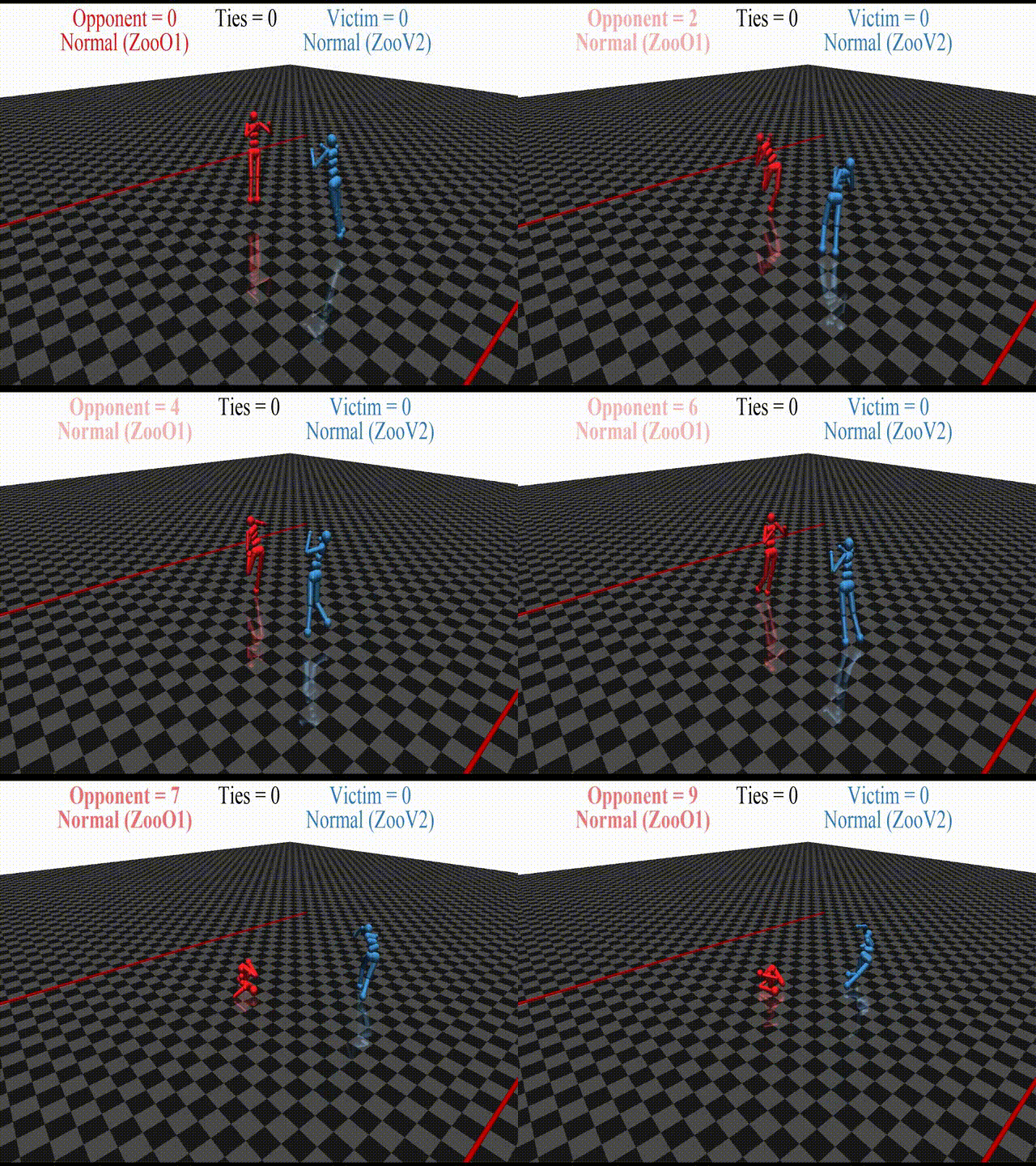
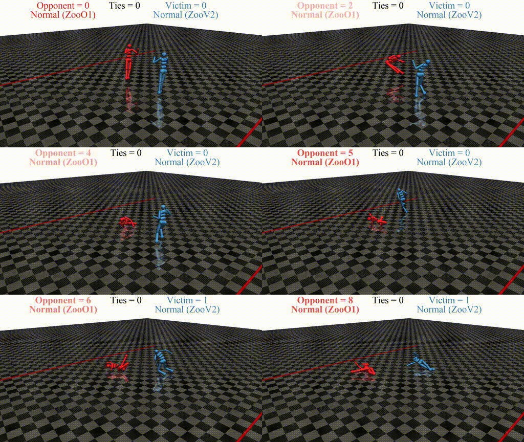
New agent (red, opponent) playing against a stock agent (blue, victim). While not even touching the victim, the opponent wins every time.
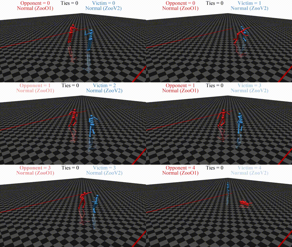
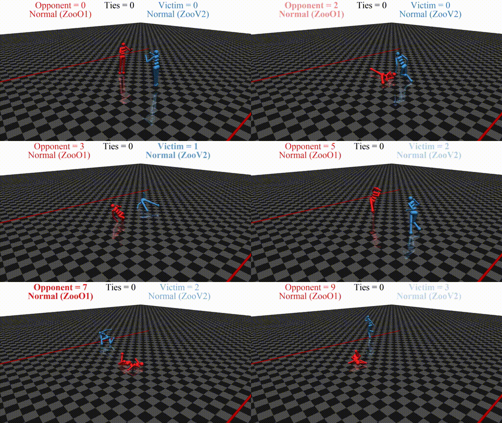
In this post, we discuss the results of my CHAI internship project aimed at discovering better defenses against adversarial policies. We consider one of the environments from the original paper: YouShallNotPass (figure above). The environment is chosen among others as the one giving the most interesting adversarial policies while staying in the Markov domain (other environments require recurrent policies). The blue player ("runner") wins by crossing the red line behind the red player ("opponent"). The red player wins by preventing the blue player from doing so. The game is zero-sum: either the red player wins, or the blue player wins. The figure below shows the "normal" behavior in this environment achieved by curriculum training by OpenAI in 2017.
"Normal" behavior in YouShallNotPass
We run defensive training in succession with training the adversary multiple times, hoping to achieve novel interesting results. Qualitative evaluation of the adversaries obtained with our method shows a diversity of novel adversarial behaviors.
Novel adversarial policy: lying on the back rapidlyNovel adversarial policy: doing splits
Background
Two-agent Reinforcement Learning
Agent-environment interaction. We consider an environment μ which allows for two agents, F and G to interact with it. The agents take actions a, and the environment responds to them with observations o and rewards r. The interaction μ↔(F,G) provides episode rollouts(histories), with episode lengthT
Average return. We parameterize agents (functions that return an action) F,G by their parameters x,y (list of matrices, for example) and write F(x) and G(y) respectively. We define RF(x,y) as the average (over episodes) return that F gets in μ given parameters x, when playing against G with parameters y, with a discount factor γ:
RF(x,y)=EH∼μ↔(F(x),G(y))T(H)∑i=1γirFi
In the same way, RG(x,y) is the average return that that G(y) obtains when playing against F(x).
The goal of RL. Informally, the goal of the agent F is to maximize RF(x,y) over possible x∈X and the goal of G is to maximize RG(x,y) over possible y∈Y, where X and Y are parameter spaces. For example, if F and G are neural networks, X and Y would be the vector spaces corresponding to weights and biases. However, this is only an informal definition, because for F it is unclear against which agent G(y) to optimize, and vice versa.
Game theory
Best response. Given a fixed opponent G(y∗), the task for F is to simply optimize
x=argmaxxRF(x,y∗)
which boils down to a single-agent Reinforcement Learning problem in a single-agent environment μ∣∣(⋅,G(y∗)): one where the agent F takes actions, and G(y∗) is "embedded" into the environment and does not change. This corresponds to the best response strategy in Game Theory: x is the best response of F to the behavior of G(y∗). Symmetrically, we can define the best response of G to F(x∗).
Note: in realistic setups, we only search over a limited space of agents, such as neural networks with a fixed architecture. Therefore, the best response becomes the best response in a class of policies.
Note: when running Reinforcement Learning algorithms, we cannot search the whole space of X and find the best response. Instead, these algorithms do a sort of local search and (sometimes, hopefully) provide a somewhat good response. We will define this more formally later.
However, which parameters y∗ (or x∗) should we choose? Let's first consider those setups that are not interesting. If a pair (x,y) is such that one of the agents can improve their performance while the other is kept constant, it means that the (ideal) training was not complete. This naturally leads to the definition of
Nash equilibrium. If a pair (x,y) is such that x is the best response to y (it cannot improve unless we change y), and y is the best response to x, it is called a Nash equilibrium:
x=argmaxxRF(x,y)y=argmaxyRG(x,y)
It was shown that Nash equilibria exist for all games (environments) under technical assumptions (although, in some games they require mixed [probabilistic] strategies).
Zero-sum games. To make things simpler, we assume that the environment is "fully competitive" or zero-sum:
RF(x,y)+RG(x,y)=0
Reward range. We additionally assume that the reward range rF∈[0,1],rG∈[0,1] and that γ=1
Comparing agents. We call RF(x,y)=RG(x,y)=0 a tie. In this case, we write x=y. In case if RF(x,y)>0, we call F(x) a winner and write x>y. In case if RF(x,y)<0, we call G(y) a winner and write x<y.
Transitive games. A two-player game is called transitive if there exist two "rating" functions sF(x) and sG(y) such that RF(x,y)=sF(x)−sG(y). Intuitively, this means that the performance of each agent is an inherent property of the agent itself.
Local Best Response. Unfortunately, computing the (global) best response in the class of all policies X is an uncomputable task, and in the case of neural network parameters X this task has no known global solution as well. An RL algorithm A can provide a somewhat good approximation to the best response using local search, given an initial point x0, the number of iterations k and the single-agent environment: x=A(x0,k,μ∣∣(⋅,G(y))). Algorithm A could be DQN, PPO, or something else.
We will write x=A(x0,k,y) meaning the same thing as above, approximate best response to the agent G(y) using algorithm A.
Since we cannot search for the best response, we need to update our definition of the Nash Equilibria:
Local Nash Equilibrium. A pair of parameters (x,y) is an Approximate Nash Equilibrium, given a probability p and a number of iterations k ifPA[RF(x′,y)>RF(x,y)]<p and PA[RG(x,y′)>RG(x,y)]<p with x′=A(x,k,y) and y′=A(y,k,x)
This simply means that, if we run the algorithm A many times from initialization (x,y) either for F or for G, we will not obtain better policies (for either of the agents), with probability at least 1−p.
Note: a (global) Nash equilibrium is also a Local one. Therefore, there exist Local Nash equilibria (under technical assumptions)
Note: the reason we have to use probabilities is that Reinforcement Learning algorithms usually include some sort of sampling step for exploration and the probability to randomly "stumble upon" any policy is thus non-zero.
Note: In our experiments, we simply run the optimization several times, thus giving a guarantee on p
Looking for Local Nash equilibrium: simplest case. To search for the Local Nash Equilibrium, we run the following procedure:
x0 and y0 are initialized randomly
xt+1=A(xt,k,yt)
yt+1=A(yt,k,xt)
More sophisticated heuristics such as training against multiple opponents at once and training against old versions of opponents are known to give better-quality solutions because they result in a "more global" search.
The problem: adversarial policies
Adversarial policies in real life: while the cucumber is no real threat to the cat, the cat is scared and avoids the cucumber when sees it, arguably, because it looks like a snake. If considered as a (no-action) policy in a two-agent environment with the cat and the cucumber, the latter "gives" an observation to the cat that scares the cat and forces it to move. This is similar to the YouShallNotPass environment: the adversary is no threat to the runner, but it forces the runner to take a specific action.
Now, let's define formally the problem of adversarial policies given all the tools we have introduced. In the simulated robotics game of YouShallNotPass (see description at the beginning of the post) we have two agents:
F - "blocker" ("adversary"), has parameters x
G - "runner" ("victim"), has parameters y
We have the initial pre-trained opponents F and G giving weights x and y. We know from previous work that the following weird stuff happens. We will write x(y1,y2,...,yn) meaning that we take agent with weights x and then train it with A(⋅,k,⋅) against a random uniform mixture of y1,...,yn. We write x<y meaning that an adversary with weights x loses against a victim with weights y
The initial agents (x,y) give a Local Nash Equilibrium, because these agents were trained against each other until convergence:
x≈y
If we run training of the adversary from scratch, we get x′=xrandom(y). This newly-trained opponent defeats the normal victim, and the policy "looks" adversarial
x′>y
If we run the training in the other direction, we get y(x′). The "defended" opponent wins against the adversary, but loses against the normal opponent - it forgets how to play against it:
x′<y(x′)<x
If we run training with two opponents, we regain the performance:
x′<y(x′,x)≈x
Now, if we run the training again, we will get another adversarial policy: x′′=xrandom(y(x′,x)) such that
x′′>y(x′,x) but x′′<y
To define how to tackle this problem, let's first understand why this might be happening.
For x′ the issue is that the newly-trained opponent shifts the distribution towards a range that the agent does not expect. This leads the agent to output nonsensical actions and fails in the game. Essentially, like in supervised adversarial examples, the agent learns to rely on spurious correlations: instead of relying on the position of the player to determine the next move, the runner includes its pose into account as well. Even if the player "physically" does not prevent the runner from winning (does not make contact), the spurious correlation that it relies on forces it to fail.
For x′′ the behavior is different, but the explanation is the same.
The agent does not even know which parts of the observation tell it about its own pose, and which about the opponent's pose. When training against a fixed opponent, the agent might start relying on other agent's features to stay upright, if it is correlated with its own pose.
So, what do we want?
In general, we would like to improve our initial victim y so that no adversary x′ can exploit it. This means that xrandom(y)≈y
A perfect solution would be a black box that outputs a policy that is dominant with respect to all other policies (does better with respect to all possible opponents). Or, at least, given an initial policy y outputs a policy y′ that is dominant with respect to y ("defends" y against adversaries).
It was shown that every game (environment) can be decomposed into transitive and a cyclic parts. Let's first figure out what we want in each of the cases
Transitive games. Example: comparing exam scores between students. Each student's performance is only determined by their skills, and there is no interaction between students. Mathematically, there exist functions determining the score for each of the players, regardless of the actions of the other player: sF,sG:RF(x,y)=sF(x)−sG(y). In this case, we simply would like to find the best x=argmaxsF(x) and y=argmaxsG(y). The pair (x, y) is a global Nash. Any freshly-trained (adversarial) policy y′ will worsen the performance of any F(x′) no less than for F(x).
Cyclic games. Example: Rock-Paper-Scissors. For all y, ∑x∈XRF(x,y)=0 and for every x, ∑y∈YRG(x,y)=0. This is a more "no-free-lunch" kind of situation: for every adversary x, some victims are better, and some are worse. For every victim ythere is a policy x′(y) that would exploit y. In this case, even if we find a Nash equilibrium, we trade off performance with respect to some opponents in terms of performance to others. Therefore, to fully specify the problem, we need to define this trade-off. We introduce a cost function c(x)∈[0,1] which defines how much y should "care" about x when optimizing for its reward. Thus, the new reward for the victim becomes RG(y)=∑x∈XRF(x,y)c(x)
In the general case, we find that our environment (YouShallNotPass) is not transitive: we found policies such that x1>y1>x2>y2>x1. This means that there are no "rating" functions sF,sG.
Before we were talking about a perfect theoretical "black box" outputting defended policies and computing attacks. Now we show that it does not exist.
For the same reason, defending against adversarial policies is an uncomputable task in the general case
Since even in the finite-computation case the AIXI (best response to an environment) is exponentially hard to compute, the problem of the adversarial defenses and attacks is as well.
We can make this setup (somewhat) realistic if we implement the Turing machines as Neural Networks (constant amount of layers corresponds to one step of the computation with tape length is the layer width).
Since we do not know if our game is (partially) cyclic, there might be no good definition of a "perfect" victim, even if we could compute it, there are only trade-offs.
A practical definition
Since we cannot assess the whole set of adversaries or victims, we define a good solution as the one satisfying the following criteria.
The victim y′ has performance with the normal opponent x comparable to y:
RG(x,y′)≈RG(x,y)
The victim y′ defeats all previously-found adversaries x1,...,xn
For a novel adversary x′(y) found during a reasonable number of iterations k, the performance of y′ does not drop significantly.
In addition, we consider the number of contacts that the adversary makes with the victim. The known adversarial policies defeat the victim without making any contact, while the "normal" opponent usually does make contact using arms and the body.
Our solution
Since the culprit of the problem is in the multitude of local minima, and there is no perfect solution, the main idea is to diversify the training procedure.
One of the methods to do so is to run population-based training: the victim is trained against multiple opponents, which are chosen from a categorical distribution at each episode: xt∼Categorical([x1,...,xk],[p1,...,pk])
Another method is to apply a regularizer during training, such as Maximal Entropy. We use both of these approaches and introduce another one.
It is known that in two-player zero-sum games with local search as an algorithm instead of best response, it is important to set properly the ratio of "strengths" between optimizers for the two agents. Here, we search over this space by increasing the time during which each of the agents is trained ("bursts")
To increase the diversity of individual opponents is to increase the exploration space of them at train time. To do so, we add the entropy regularizer to the training loss, so that policies are encouraged to give uncertain predictions. This makes the policy take more random actions, and thus explore the environment better.
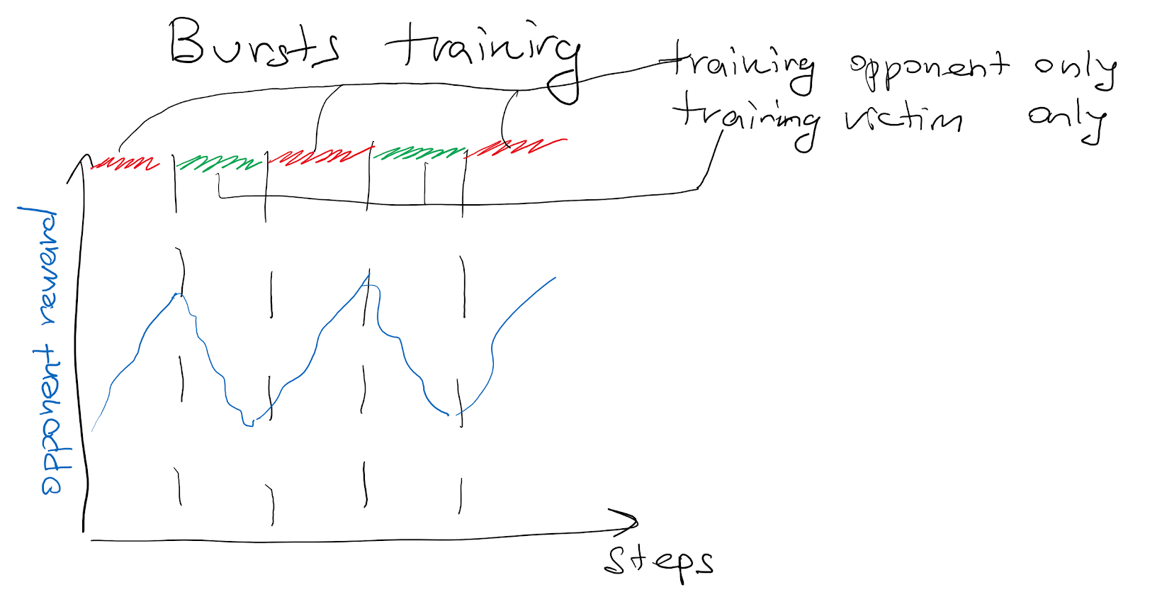
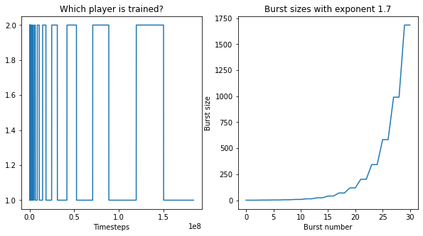
In addition, we note that traditionally, both agents are trained at each iteration, which gives every individual agent little time to come up with a good response. Ideally, we would like each agent to find the best response policy to all other agents at each iteration. However, since RL does not give optimal solutions even with infinite iterations, we simply increase the number of steps for each agent. We approximate the best response better by giving each policy more time when the other one is frozen. We call this training in bursts. To search for the optimal burst size, we give more and more time for each policy to develop the best response, given the other policy. We increase the burst size exponentially.
Expected rewards in the bursts approachSummary of the bursts approach
To sum up, at the beginning of each episode, we select the 'normal' opponent with probability pnormal=1/2, and otherwise, we sample from the set of randomly initialized adversaries {xadv.i}Ki=1. Therefore, the victim's return that is being optimized is the following linear combination of previously-defined returns with a single opponent:
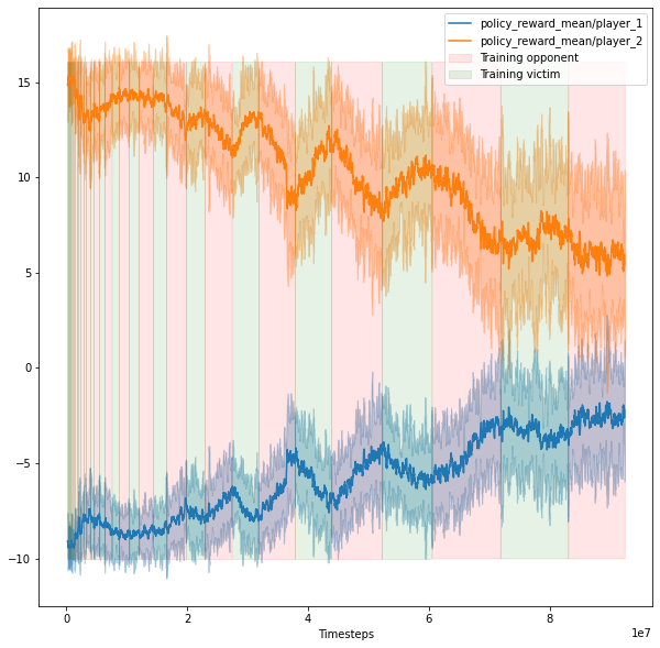
The following chart illustrates one trial with bursts training, 1 adversary, and 1 normal opponent. The red background represents training the opponent, and the green background corresponds to training the victim. The orange curve is the victim's reward, the blue curve is for the adversary's reward, and the green curve is for the normal opponent's reward.
Experiments ran:
1. Previous results (training opponent, then victim, then opponent again)
2. Bursts for 2 opponents ("PBT1").
3. Bursts with a normal opponent and adversarial opponent with p=0.5 ("PBT2")
4. Bursts with a normal opponent, 5 adversarial opponents, p=0.5, and entropy coefficient ("PBT5")
Training with bursts with 1 victim and 1 adversary. The background shows which policy is currently trained. The orange curve is the reward for the victim, and the blue curve is the reward for the adversary. Generally, the reward of the player that is currently trained is increasing.
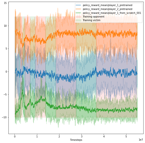
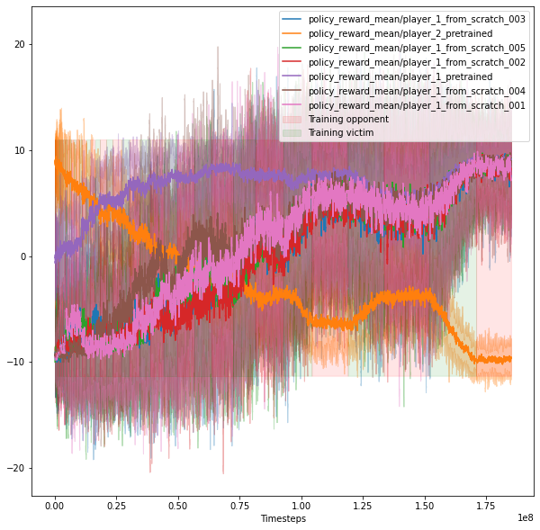
Training with bursts with 1 victim (orange), 1 adversary (green), and 1 frozen "normal" opponent (blue) from the OpenAI paper. At the beginning, the reward of the adversary increases and decreases, depending on which agent is trained. After that, all rewards stabilize and do not change significantlyTraining in bursts with 1 victim (orange), 1 normal opponent (light blue), 5 adversaries (the rest). The training curves are quite strange: first, the victim's reward sometimes does not increase even when it is being trained. In addition, the victim loses at the end. We explain it by the fact that the victim has to defend against 6 different policies, which is hard, because the architecture of the victim and each adversary is the same.
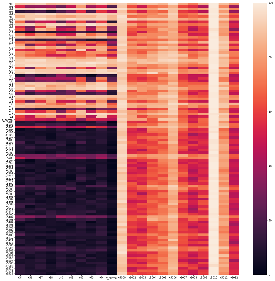
The evaluation shows that victims from the PBT5 experiment (see the description above) are easy to defeat by adversaries both from the PBT2 experiment and the PBT5 experiment. In the same way, the adversaries from the PBT5 experiment do not win against the victims from the PBT2 experiment. This shows that the PBT5 experiment failed to provide strong victims or adversaries. Therefore, we discard data from this experiment in the following analysis and only analyze the PBT2 experiment.
(click to enlarge) Heatmap of the win rate for the opponent for all victims and opponents from PBT2 and PBT5 experiments. v04-v44 are the victims (columns) from the PBT2 experiment, vnormal is the "normal" victim from the OpenAI paper, v5000-v5012 are the victims from the PBT5 experiment. Adversaries (rows) a00-a44 are from the PBT2 experiment, anormal is the normal opponent from the OpenAI paper, and adversaries a5100-a5512 are from the PBT5 experiment. For the latter, the index 5xyy indicates x - number of the adversary in the trial and yy -- the number of the trial.
Results:
1. Training in PBT0 shows that the reward oscillates between the opponent winning or the adversary, there is no convergence. In PBT1, the rewards stabilize. In PBT5, the victim generally loses.
2. In PBT5, we see some novel behaviors (using hand to knock down the victim, splits, sitting and jumping, falling on the back or on the side). The burst size does not correlate with the robustness. The game is non-transitive: there are loops in the graph of victories
Graph of victories
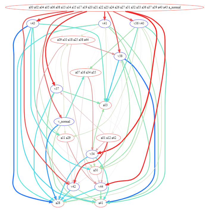
We interpret the win rate table as a graph with all policies as nodes, and a directed edge between policies indicating that the parent wins when playing against the child.
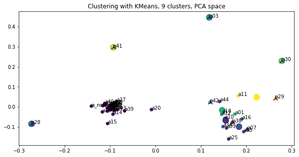
We cluster the nodes based on the similarity of their win vectors against all possible opponents to reduce the dimensionality. We select the closest policy to the cluster center to represent the win rates of the cluster.
Clustering of adversaries based on their win rate vectors w.r.t. all victims. Named dots are the adversaries, big dots are the cluster centers, and the marked adversaries are the ones that are closest to their centers.
The green edges indicate that the victim wins, and the red edges indicate that the adversary wins. The edge width represents how far away from 50% is the win rate (the thickest edges are either 0% or 100%)
Graph of victories for clustered policies in the PBT2 experiment. We see that a set of strong adversaries (at the top)
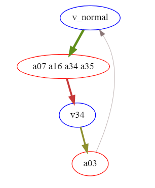
The graph contains cycles with low strength (distance from 50% divided by 50%), minimal strength in the cycle is 8%
Behavior analysis: contacts and win rate
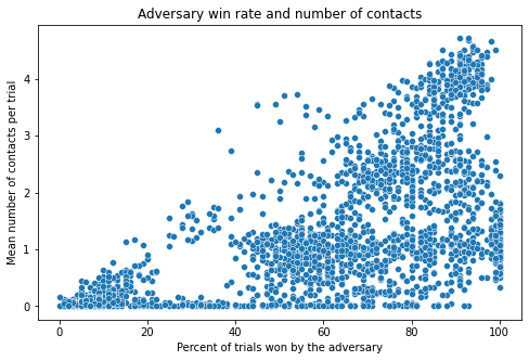
We collect all the policies from bursts training and evaluate them against each other in terms of win rate and the number of contacts the players make. The results show that there is in general a group of agents for which the contacts determine the win rate. These win by physically making the victim trip and fall. Another group wins without making any contact: these are the adversarial policies in a proper sense.
Number of contacts and the win rate for all the pairs of victims and opponents from bursts training. The group with contacts=0 at the bottom consists of properly adversarial policies.
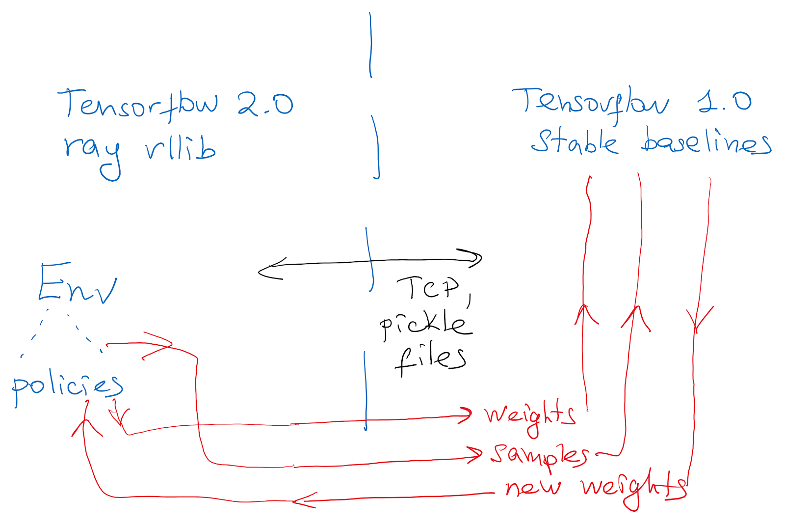
We use ray and rllib because of their good multiagent support. We import Stable Baselines policies for the multicomp environment by creating a Keras model matching the original architecture and loading the weights. To check the correctness, we compare the outputs of both networks on a set of random inputs.
However, it turned out that rllib's PPO performance was not enough to match that of the original paper. Therefore, we use Stable Baselines as the trainer and rllib to collect data. We connect frameworks via TCP like in the diagram below:
Additional experiments
We try linear policies with the rllib PPO trainer. They do not give high returns. Interestingly, linear policies result in qualitatively different behavior.
We try tf-agents and rlpyt frameworks, but they do not give higher rewards than rllib
We try python-neat evolutionary strategies and random search with a constant policy. They do not give higher rewards than rllib
We try lower and higher network sizes, resulting in [64, 64] being the optimal one.
Conclusion
Adversarial policies (AP) are a novel topic in the field of Adversarial Machine Learning. Instead of crafting a specific observation, like in (supervised) adversarial examples, here, the goal of the adversary is to develop a policy that would give such observations. Defining what is an AP is a bit tricky and depends on the environment. Prior work shows that there are adversarial policies that win without even touching the opponent.
1. In this project, we search for better defenses against AP and find a variety of novel adversaries with diverse behavior
2. We empirically prove that the YouShallNotPass game is not transitive, as we find cycles in the win graph.
3. In addition, we include the number of contacts the agents make into the definition of an adversarial policy in the YouShallNotPass environment
How to help the field
Right now, there are a few bottlenecks leading to slowdowns:
Lack of a coherent definition of an adversarial policy. To alleviate this, it is worth studying this phenomenon in a wider range of environments
Simple environments. While MuJoCo environments lead to adversarial policies because of diverse possible behavior, these environments are high-dimensional and hard to simulate. Finding environments which are complex enough to allow for adversarial policies yet simple enough to speed up training would increase training speed
Efficient implementations. The current sampling speed in RLLib with our implementation is around 400 samples per second on 1 CPU, which is much lower even than the environment's speed (1000 steps per second)
Current RL agents are prone to catastrophic forgetting. If we could remember the adversaries and our local best response to them, we could match the current behavior to the closest adversary from memory, and then give our best response. In addition, we can learn models of adversaries and "bootstrap" their actions, in case if it is important to be robust to a novel adversary that we have never seen and made the fewest amount of mistakes.
1
More posts like this
92
Focus on the places where you feel shocked everyone's dropping the ball