Comments
Persistence and reversibility – long-term design considerations for wild animal welfare

45 min readJan 28, 2020
38


Crossposted from the Wild Animal Initiative blog.
When designing interventions to improve the welfare of wild animals, we want to maximize the expected benefit produced given the cost.[1] A major factor in the cost-effectiveness of interventions is the persistence of the effects. The longer they last, the higher the ratio of benefit[2] to cost, all else being equal. However, due to widespread uncertainty concerning the effects of our actions on wild animal welfare, it is possible that an intervention will turn out to do more harm than good. Reversibility can contribute to cost-effectiveness by allowing bad outcomes to be reversed, limiting the damage of an intervention gone wrong. In short, we want to optimize persistence given a good outcome while still preserving option value in case of bad outcomes. However, there is a tension between persistence and reversibility, since most factors that contribute to high reversibility will also lead to low persistence, and vice versa (Table 1). This report aims to explore the importance of persistence and reversibility to wild animal welfare interventions, how to negotiate trade-offs between them, and ways to sidestep the trade-off altogether.
My main conclusions are:
Strictly speaking, no action can truly be undone or fully reversed. Even after a thorough effort to undo an action, the resulting world will inevitably be at least slightly different from the counterfactual world where the original action never occurred. Thus, rather than expecting complete reversal, a more reasonable objective might be to minimize the differences between the world where the action was reversed and the world where the action was never taken.
While the state of the world that maximizes utility might not necessarily correspond to either the reversal or no-reversal world (see Appendix A), reversibility can serve as a good approximation for how to incorporate option value into the prioritization of wild animal welfare interventions (cf. Schubert & Garfinkel 2017). For the purposes of this report, I define it as:
Reversibility: The fraction of the effect of an intervention that should be reversed (r) so as to maximize the expected utility of a reversal (see equation 1), given a bad outcome.
Even if an intervention with poor results could be reversed to a high degree with sufficient effort, the optimal strategy may not be to attempt the full reversal. This is because there might be other valuable actions that could be taken using the time, money, and other resources spent on reversal.[3] To understand why, consider the following example:
Box 1: Damming a river example
Imagine we dam a river in order to create more wetland habitat. Later, we realize that this was a bad idea, and that things were better before we flooded the area, so we attempt to reverse the intervention. Removing the dam is easy, and 95% of the flooded area drains right away. But there are still small ponds in 5% of the area we wanted to drain, because there are low-lying areas that do not drain back into the river. To continue to reverse the flooding, we’d have to bring in heavy machinery to dig canals that transport the water away. We might then decide that such an effort would not be worth it, if the financial cost of digging canals is greater than the utility of draining the last 5% of the land. In this case, we would say the point of optimal reversal is 95%, so the original river dam intervention turned out to be 95% reversible.
We can formalize the foregoing intuitions as follows: to maximize expected utility, the fraction “r” of some intervention A (e.g. damming a river) that one should try to reverse when a bad outcome occurs is given by the utility gained by reversing the intervention, minus the utility lost in the form of an opportunity cost. This cost is caused by not investing in some intervention B, where intervention B is the possible action with the next highest expected utility (compared to further reversing A).[4] The utility-maximizing fraction r can be described by the following equation:
Box 2: Equation 1, defining optimal reversal fraction
EU_reversal = max_r(r × V_r=1 − C_r × CE_intervention_B)

Where

EU_reversal = maximum expected utility produced by the reversal

r = the fraction of a total reversal that is undertaken

V_r=1 = the total amount of utility that would be produced if we assume that a full reversal could be undertaken

C_r = the cost of reversing the intervention by amount r

CE_intervention_B = the cost-effectiveness of the next best action (intervention B)
As the damming example illustrates, there are probably diminishing returns to increasing r due to the increasing costs of reversal (C_r ; see Figure 1), such that it might become increasingly costly to make marginal improvements on r as r increases.[5] Therefore, max_r is included in order to find the value of r that maximizes expected utility, where an increase in r from that point yields a lower expected utility. Equation 1 represents the optimal balance between when to keep reversing the effect of an intervention, and when to cut your losses and not invest in reversing the intervention any more, given that continuing the reversal is more costly than other things that you could use your resources for.[6] The definition of reversibility is somewhat similar to social-ecological resilience (e.g. Adger et al. 2005), although reversibility here relates to both human and (wild) animal well-being. For information on how the definition of reversibility relates to the value of information and the cost-effectiveness of an intervention, see Appendix A.
Intuitively, comparing financial costs to wild animal welfare benefits might seem odd—we might, for instance, wonder if it is even possible to assess the price of animal wellbeing. For decision-making purposes, however, we can ask a simpler question instead: Is there a way to improve welfare more with the same resources? Stated differently, we want to know the opportunity cost of spending resources on a particular project.
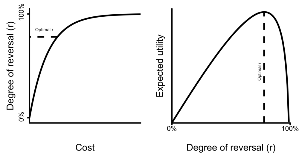
Figure 1. Hypothesized relationship between cost of reversal and degree of reversal (left), and the resulting function describing expected utility (right). Expected utility combines the costs and benefits of reversal into one single metric. The optimal degree of reversal is thus the r for which the expected utility is maximized.
Our empirical understanding of the world generally improves over time. For example, empirical information about biological systems has fairly reliably increased over time in recent years,[7] as has our ability to process large amounts of data.[8] In the future, we will probably know more about how to effectively improve wild animal welfare than we do now. Reversibility allows us to take advantage of new knowledge by making it easier to change course if we discover that an intervention is actually suboptimal.
What these facts indicate is that the value of information about the effects of wild animal welfare interventions is likely high.[9] Value of information is generally higher the more uncertain the utility of the action is, the cheaper new information is to gather, and the more time we have to reap the benefits of acting on new information. These conditions seem to hold for wild animal welfare interventions. Right now, we know very little about how to reliably improve wild animal welfare, so the effects of our actions will often be uncertain. But the fact that wild animal welfare has received so little attention also means that there are probably high marginal returns to targeted research on the subject, making new information relatively cheap. Even in the absence of a research program dedicated to welfare biology, an increased understanding of ecology in general will be very useful for wild animal welfare interventions. The positive or negative consequences of interventions could last for decades, so the impact of reversing a suboptimal intervention could easily justify the cost of information gathering.
Just as empirical knowledge can improve, perhaps moral reasoning can improve. Looking back in time, humanity's moral circle has gradually expanded to include ever larger groups of individuals (Singer 1981; Roser 2019). Just as our ancestors overlooked moral atrocities like racism and sexism, perhaps present humans also have moral blind spots that future humans will find. The more likely we think this is, the more valuable reversibility becomes, because future generations will have a better understanding of moral philosophy (MacAskill MS-a).
However, rather than achieving some idealized version of our current values, it is also possible that future humans stray away from our values in ways that we would not endorse (MacAskill MS-b). If this happens, reversibility is not a strength but rather a weakness, because any progress we do make is easier for antagonistic decision-makers to undo. For example, if future generations stop valuing the well-being of humans of a certain ethnicity, they might reverse earlier actions such as the Universal Declaration of Human Rights. This would constitute a value loss from the point of view of the morals of current humans.
I have so far described human values as a unified entity, but most human actions that affect wild animals are motivated by disparate and ever-changing goals, almost none of which are aimed at improving wild animal welfare. If this continues to be the case, it is possible that future actors will, intentionally or unintentionally, reverse the effects of interventions even if they are net positive from the perspective of our current values.
All else equal, reversible interventions will probably be easier for the public to get behind, because non-reversible interventions might be perceived as too risky. This could dominate other considerations: even when a hard-to-reverse intervention is preferable to a reversible intervention, a reversible intervention is probably preferable to no intervention at all. Consequently, I take the tentative working hypothesis that reversible interventions are preferable to non-reversible interventions, especially in the wild animal welfare space where uncertainty abounds.
I define persistence as:
Persistence: The expected duration of the counterfactual effects of an action.
Here, the duration of an intervention refers to its mean lifetime. If an intervention’s effects decay exponentially over time, duration is proportional to the half-life of the decay function. The word “counterfactual” in the definition is also of key importance, as the persistence of an action is only compared to what would otherwise have happened. For example, if we plant a forest in a field, but a forest would have established itself in the same field without our help 25 years later, then counterfactually we can only claim credit for the first 25 years of the intervention’s effects. Furthermore, interventions are persistent only when they are independently so.[10] Refilling a bird feeder once a month would be classified as a low-persistence intervention, as even if we refill the feeder for many years, the effects of each discrete filling event only lasts for a short period, and the intervention would not persist without upkeep.
Using the terminology of dynamical systems theory, highly persistent effects can be described as attractor states[11] (Brin & Stuck 2002), which are possible to enter but difficult to leave (cf. absorbing states in Greenwell et al. 2003, and path dependence in Mahoney & Schensul 2006). Highly persistent states generally represent deep or wide basins of attraction.[12] To understand the relationship between persistence and the expected utility of our actions, consider a curve representing the utility of an intervention over time. Whether or not the expected utility of an action is positive, the distribution of expected utility per unit time is probably best represented as an exponential decay function,[13] representing the survival of intervention effects over time. The overall utility of the intervention is represented by the integral over time, and depends on both the effect size per unit time (i.e. the utility of the intervention at each time point), and the width of the distribution (i.e. the duration of the interventions effects). Persistence influences this latter factor: the more persistent an intervention, the wider the distribution.
As may already be apparent, persistence and reversibility are closely related. Reversibility is one factor that determines persistence, as an intervention that is reversed would be less persistent than one which is not. Critically, both reversibility and persistence are relative to human capabilities. Some interventions will be reversible only if certain technological advances are achieved. Similarly, some interventions will be persistent only if certain abilities are not achieved. However, note that just because future humans can affect the persistence of our actions, does not mean that they will.[14]
As discussed in the section Costs and benefits of reversibility, reversible interventions seem preferable, as they are more politically feasible and they preserve option value. Furthermore, if future humans are unable or unwilling to reverse the effect of an intervention, a persistent intervention is beneficial when the intervention has positive effects in expectation, because the expected benefits will last longer.[15] Thus, we want to find interventions that are reversible when humans are moderately to highly capable, but also persistent in situations where humans are not interfering with the interventions, for whatever reason (i.e. we should prefer the solid intervention in Figure 2). I will refer to such interventions as being persistent in the face of natural processes. If human capabilities decreased or became virtually non-existent, such interventions would have a comparatively high persistence. Thus, the importance of long-term persistence depends on the future prospects of humanity. Relatedly, it seems that if the likelihood of reduced future human capabilities is high, the utility produced by implementing reversible interventions becomes comparatively low.[16]
One way in which human capabilities could be drastically reduced is if we go extinct. Consequently, knowing roughly how likely extinction is will probably be useful when assessing the value of reversibility and long-term persistence in the face of natural processes. According to researchers studying the risk of human extinction, the probability that humans will go extinct in the next century is quite high,[17] perhaps as high as 19% (Sandberg & Bostrom 2008). Even if we think that this latter estimate is an overestimation by an order of magnitude (i.e. if we think that the real estimate is closer to ~2% risk per century), it still makes sense to account for this possibility when making decisions on interventions designed to help wild animals.
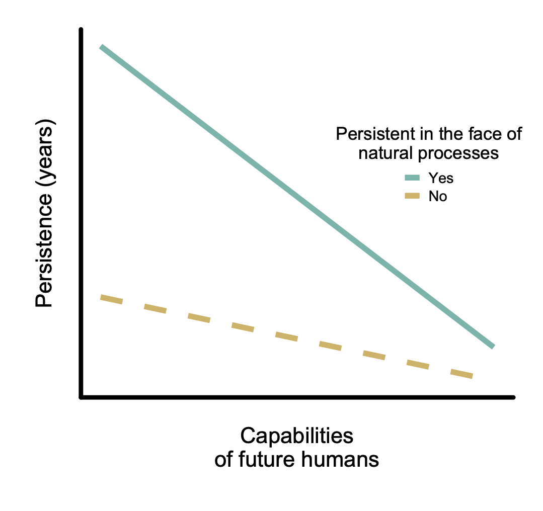
Figure 2. Two hypothesized relationships between expected persistence of interventions and the capabilities of future actors. Each line represents a hypothetical intervention that is either persistent in the face of natural processes (solid teal line) or not (dashed mustard line). Both lines represent interventions with high reversibility when future capabilities are comparable to current human capabilities (a non-reversible intervention would be represented by a straight horizontal line regardless of persistence). That the two lines approach each other with increasing capabilities is mainly based on the assumption that high future capabilities will lead to more ambitious rearrangements of the natural world, largely without wild animal welfare in mind, causing average persistence to be low.
As the number and degree of the changes caused by an intervention grows, the more likely it becomes that the results of those changes will be persistent and hard to reverse. Such considerations about projects that are larger in scale is one reason to pilot small-scale tests when possible. The scale of an intervention encompasses the sum total of its effects, including its geographic scope, the number of animals affected, the size of the impact on each animal, etc. For a more thorough discussion of what is meant by scale, see Appendix A (Granularity of world-comparisons).
One reason large-scale interventions might be more persistent is that they are more likely to pass thresholds where negative feedback becomes positive feedback, making reversal considerably harder. By definition, a threshold is dependent on the magnitude of the change in the parameter value(s). If you go above or below a certain value, you move towards a new state, which can be more or less persistent. It is thus inherent to threshold effects that the probability of reaching the threshold is dependent on the size of the shift in the parameter. Large-scale interventions induce larger shifts in parameter values than small-scale interventions of the same type. Hence, the likelihood of transgression of an arbitrary threshold increases with the scale of an intervention.
Political feasibility is one of the most important factors to consider when balancing the persistence and reversibility of wild animal welfare interventions.[18] Interventions that are persistent in the face of natural processes are likely to be met with greater public opposition, although making sure that such interventions are also highly reversible might mitigate some of this opposition. Even though humans have long been altering ecosystems on a massive scale to meet our needs (e.g. Barnosky et al. 2011; Steffen et al. 2011; The World Bank 2016), explicitly stewarding nature for specific purposes might be perceived negatively by the public (e.g. as with GMOs in Europe: Eurobarometer 2010). In other words, certain interventions might superficially seem very cost-effective, but only in the absence of political and coordination costs. If public opposition to these interventions are large enough, the cost-effectiveness of working towards implementing them will be low.
Based on the above discussion, we should prefer interventions that are reversible given current human capabilities, fairly persistent in the face of natural processes, and initially restricted in scale. In the following sections I will apply these ideas and highlight good and bad concrete examples.
We should generally expect interventions with high reversibility and high persistence in the face of natural processes to be unusual, since the factors that make interventions persistent in the face of natural processes are often similar to the factors that make them persistent despite deliberate human action (i.e. low reversibility).
After further development, gene drive technology has the potential to become an exception to this rule. It is important to note, however, that any immediate use of gene drives in the wild would likely be highly negligent. Safety measures have to be perfected and extensive laboratory testing performed (Min et al. 2017; Dhole et al. 2018) before such an implementation.
A gene drive is a process that occurs when a specific genetic element consistently increases in frequency in a population, even if it does not confer a fitness benefit to the individuals that carry it. Gene drives have existed naturally for millions of years,[19] but scientists have recently discovered ways of creating engineered gene drives using the tools of CRISPR/Cas9 (Esvelt et al. 2014).[20] CRISPR/Cas9 is a highly precise gene editing tool, originally discovered in prokaryotes, where it serves a function in acquired immunity (Jinek et al. 2012). CRISPR/Cas9 can be constructed to constitute a gene drive, spreading almost any desired genetic change. Gene drives increase the probability of spreading the gene drive complex from the usual 50% per offspring (so-called Mendelian inheritance) to almost 100%.
Gene drives are probably highly persistent, because they enable a gene to be passed on until all members of a species have it. It is possible that over time, natural selection would “undo” the effects of the gene drive, as presumably the original phenotype was better for evolutionary fitness. However, even with unfavorable fitness effects, a gene drive complex could last for at least a few hundred generations (Noble et al. 2017). The type and scale of the gene drive is relevant to persistence. For instance; deleting a whole gene will probably constitute a more persistent modification. Such a change will likely be less affected by mutation and selection than simply modifying the sequence of an existing gene, because mutation and selection can bring the previous function back if the gene was not deleted. Furthermore, if there are few homologous genes that could be co-opted to perform the function of the deleted gene, it could take a long time to regain the function that the deleted gene provided. Lastly, modifications that become fixed[21] for the whole species are also likely to be more persistent, as there is less variation in the population for natural selection to act upon.
Genetic modifications to wild animals using gene drives could have long-lasting effects on wild animal welfare[22] (Johannsen 2017). If reliable and safe gene drives are developed, it will likely be possible to make many previously proposed interventions to improve wild animal welfare more persistent in the face of natural processes. For example, gene drives could help reduce parasite loads on wild animals (Ray 2017) or nonlethally prevent overpopulation by reducing fertility (Brennan 2018).
Depending on how they are used, gene edits might be detrimental to the long term viability of a species. Artificial alterations of a species’ traits will push the distribution of trait values away from their current fitness optimum (as there is no reason to edit genes if no functionally relevant trait is altered). Furthermore, a population might spontaneously go extinct if the population size is suppressed below a certain non-zero number, for instance if the population growth rate becomes negative (so-called Allee effects), where the alternative stable state is extinction (Dennis 1989; Beisner et al. 2003). The effect of reduced fitness and an accompanying drop in population size could thus be an increase in the extinction rate of gene-edited species.
Extinction could also be intentional. Screwworms were eradicated in North America (Vargas-Terán et al. 2005), and some people have proposed eradicating malaria-carrying mosquitoes (Matthews 2018). Eradicating a species would have high persistence in the face of natural processes (see Extinctions below).[23] It is currently impossible to bring species back from extinction, and reversing the welfare effects by other means would probably be very hard. Thus, to reduce the probability of unintentionally causing a species to go extinct, the first field trials of gene drives (after rigorous laboratory testing) should ideally be conducted on isolated (Webber et al. 2015) and non-threatened populations, since larger populations are generally less vulnerable to extinction (O’Grady et al. 2004; Fagan & Holmes 2006).
Despite being persistent in the face of natural processes, gene drives might be highly reversible[24] by humans (Oye et al. 2014; Min et al. 2017). Although none are currently ready for use in the field, there are several gene drive reversal methods currently under development (Min et al. 2017; Noble et al. 2019) that, in combination, could allow for the suppression of the spread of a gene drive (although issues still remain; see Girardin et al. 2019).
One potential method would be to release a second gene drive that targets the first gene drive, which would then reverse whatever genetic change had been previously implemented. However, such a gene drive would still leave traces of the second gene drive in the population, because the CRISPR/Cas9 machinery would remain. Although this would likely have little effect on the ecosystem or the welfare of the animals, a way of removing all traces of the second gene drive is also under development (Min et al. 2017). If this alternative method is successfully developed, it would be significantly more complex than current gene drives. It would require the release of different types of genetically modified organisms at different stages, using underdominance[25] and so-called daisy drives[26] to prevent fixation of the gene drive elements (Min et al. 2017). Furthermore, to remove all traces of gene editing, the population(s) could be subjected to a genetic bottleneck. In such a scenario, the offspring of the (possibly few) remaining wild-type individuals would constitute the future population (Min et al. 2017), and this population would thus experience a loss[27] of the genetic diversity present in the individuals who carried the gene drive. However, new genetic diversity would be regained given enough time, which would be the type of reversal that we care about (see Appendix A for a discussion about the choice of metric for reversibility).
Currently available gene drives will spread continuously through the population until the gene reaches fixation. Through migration, the gene could spread to all non-isolated populations of the same species. Developing localized gene drives would help avoid these large-scale effects. This would maintain local sovereignty by giving communities the ability to opt out of the use of gene drives when they are deployed nearby. Currently proposed methods for localizing gene drives are far from implementation-ready. They seem either prohibitively expensive or too likely to spread to neighboring populations (Esvelt et al. 2017; Dhole et al. 2018), although there is no reason that such hurdles could not be overcome with future innovations.
The underdominance-coupled daisy drives mentioned earlier (Noble et al. 2019, Min et al. 2017) might be another way to reduce the geographic spread of gene drives. The daisy drive system would limit the number of generations during which the gene drive can spread by breaking down the self-replicating machinery into separate units that are dependent on each other (Noble et al. 2019). Crucially, the primary unit is introduced as a normal gene without the same ability to spread throughout the population as the other elements have (Noble et al. 2019). Since there is one component that segregates naturally in the population, and is necessary for driving the next component in the daisy chain, it should eventually be purged from the population by natural selection. This will happen to all elements of the daisy drive that have not reached fixation; when the element that drives them disappears, they will be weeded out by natural selection as well. This process ensures that the daisy drive, if constructed properly, will have reduced persistence, potentially allowing future researchers to implement small field trials after sufficient laboratory testing. These developments are important especially considering the negative public perception of genetic modification, where more work on the possibility of controlling the spread of gene drives might mitigate some of this anticipated opposition.
The avoidance of irreversible actions can be considered a type of highly reversible intervention. The parallel is imperfect, because the “intervention” here is the deliberate avoidance or delay of another intervention. But the benefits are similar. If the action can be undertaken just as easily in the future, then avoidance can easily be “reversed” by taking the action at a later date.
In other words, delaying irreversible actions preserves option value. If irreversible negative effects are possible, then accounting for option value can flip the sign of the expected utility of an action. In general, avoiding entering persistent states that are hard to exit seems like a good heuristic (Schubert & Garfinkel 2017). This will be a more reliable guideline in cases with high uncertainty about the action’s effects and low costs to delaying the action.
Below, I describe three actions with low reversibility, high persistence, and uncertain utility. These are cases where we might prefer avoiding the action in order to avoid highly persistent negative effects.
The local or global extinction of a species[28] seems to be particularly persistent and hard to reverse, even if we are looking only at the effects on wild animal welfare. However, it is possible that closely related species will fill the functions of the extinct species fairly quickly (Oliver et al. 2015), counteracting the effects of extinction and potentially lowering the persistence of the effects on animal welfare. For example, the extinction of a parasite might temporarily improve the welfare of its host species, but the welfare effects would be counteracted if a new parasite filled the niche left behind.
Below I discuss the factors that influence the likelihood of such replacements, and to what extent the replacements can be thought to nullify the effects of extinctions. I mainly focus on local or global extinction of multicellular organisms rather than pathogens and other microorganisms, although some concepts and ideas will certainly be transferable.
The competitive exclusion principle prohibits the stable coexistence of two species with exactly the same ecological niche because one would outcompete the other (as described by Lotka-Volterra models of competition: Gotelli 2001, p. 112; Cushing et al. 2004). In reality, there are almost always slight differences in niches, even for highly similar species. In general however, there seems to be functional redundancy in ecosystems where the function of an extinct species is often taken over by some other species (Oliver et al. 2015), although the probability of functional replacement seems to depend on biodiversity and functional homogeneity, among other things (Fonseca & Ganade 2001; Solé et al. 2002).
The probability of such replacements are also related to the concepts of fundamental and realized niche. A realized niche is the niche that is currently occupied by the organism. In contrast, the fundamental niche is the niche that is theoretically inhabitable in terms of abiotic factors if the interactions with other species had been different,[29] for example, under less competition with other species for that niche space (Hutchingson 1957; Soberón & Peterson 2005; Holt 2009). Species distributions are often constrained by interspecific interactions (Ricklefs 2010),[30] which might lead to colonization of new niches if interspecific competition is relaxed.
It is likely the case that vacant niche spaces could be occupied by many different species. If an extinct species fed on many different types of plants, for instance, these plants might in the future be consumed by several different species. Even if the niche replacement by competitors is imperfect after an extinction event, selection would act on the species that had partially replaced the extinct species, ultimately filling the niche completely (cf. adaptive radiations: Stroud & Losos 2016; Cooney et al. 2017). The more closely related the replaced and replacing species are, the more probable it is that the replacing species would have pre-adaptations that would allow it to move into the extinct species’ phenotype space. The generation time of the replacing species is also important, because together with other factors such as population size and genetic diversity, it determines the rate at which the occupying species can adapt to the available niche space. Future work on niche replacement and functional redundancy would likely reduce the uncertainty in terms of the persistence of the welfare effects of extinction events.[31]
In cases where niche replacement is very unlikely or impossible, the average length of the existence of a species is a reasonable upper bound on the estimate of the effects of species extinctions, at least in the absence of human activity. The average lifespan of a species is estimated to be in the vicinity of a couple of million years.[32]
Although climate change is of course not an intentional wild animal welfare intervention, reflecting on the persistence and reversibility of global warming can help shed light on how its effects might influence animal welfare over generations. Many of the persistent effects of climate change will influence wild animal welfare,[33] although the precise nature and value of those effects is unclear.[34] For some species or populations, it is for instance possible that a warming climate could even cause beneficial changes, such as shorter winters and greater food availability. In the case of humans, the welfare effects are almost certainly negative, which could in turn prevent humans from acting to help wild animals.[35]
Anthropogenic carbon emissions can have long-lasting effects on earth’s systems. Between 65% and 80% of current marginal CO2 emissions that are released into the atmosphere will remain there until they are absorbed by the oceans, a process that will take somewhere between 200 and 2,000 years (Archer et al. 2009). The remaining 20% to 35% of atmospheric CO2 will be absorbed by ocean sediments as CaCO3 over tens of thousands of years (12,000 to 45,000 years, Archer et al. 2009).[36] However, these estimates of how long CO2 persists in the atmosphere describe the persistence in the face of natural processes. What timescales are reasonable given predictions about human activities? In other words, how reversible is climate change?
The presence of excess CO2 in the atmosphere mainly brought about by the burning of fossil fuels seem hard to reverse currently, but if we scale up carbon capture and storage (CCS) quickly enough, it may turn out to be fairly reversible relative to its scale (IPCC 2005, p. 12).[37] It is at least plausible that improvements in CCS technology, or some unknown future technology, could substantially reduce the CO2 concentration in the atmosphere within this century, although reversing ocean acidification and the melting of ice sheets might take a lot longer (Grant et al. 2014; Mathesius et al. 2015).
Although CO2 concentrations may be reversible, their effects may not be. Climate change contributes to an increased rate of extinction (~10% of all species might be lost, Urban 2015) and other seemingly persistent changes, which would have unclear effects on wild animal welfare. Therefore, the results of climate change overall are harder to reverse than the mere increase in the concentration of CO2 in the atmosphere. Thus, it seems that the persistence of the effects of climate change will likely be fairly high, even in the face of human attempts to reverse the effects.
Energy efficiency enhancements that lead to increases in organisms’ absolute fitness are likely highly persistent, because evolution will tend to preserve and spread beneficial changes. Human actions can facilitate changes in traits that natural selection cannot, by forcing transitions across deep fitness valleys. Such modifications are currently under development in plants[38] using respiratory bypass, where inefficiencies in the photosynthetic machinery can be removed in crops using genes from bacteria (South et al. 2019).[39]
If such improvements spread to wild plants, for instance via species hybridization (Warschefsky et al. 2014), it could lead to a large increase in biologically available energy. Because plant productivity increases with increased incoming solar radiation (Nemani et al. 2003; Wright & Calderón 2006; Graham et al. 2003; Dong et al. 2012),[40] we would expect increased photosynthetic efficiency to have the same effect. Furthermore, future speciation events could spread the changes further, leading to a large shift in the global composition of plant species. This could lead to substantial increases in global biomass and biologically available energy, which could have large implications for wild animal welfare by generally increasing wild animal populations.
Although the extent of the influence of greater plant biomass on animal populations likely depends on the extent to which a population is resource limited (Power 1992), several studies have shown that food supply and experimental supplementation is correlated with larger animal populations in multiple taxa (Dempster & Pollard 1981; Prevedello et al. 2013; Ruffino et al. 2014; Curtis et al. 2015). However, it is unclear how well these isolated effects on individual species translates into an overall effect of enhanced photosynthesis across the board.[41] Generally, all animal populations have upper limits set by negative density dependent effects (cf. Malthusian trap[42]) where increases in resource availability could lead to increases in population size if the carrying capacity is increased (Hixon 2008; Huston & Wolverton 2009; but see the paradox of enrichment: Jensen & Ginzburg 2005). Whether such potential increases in the number of wild animals are good will depend on, among other things, questions of population ethics (e.g. Greaves 2017) and the balance of suffering and happiness in nature (Horta 2010; Groff & Ng 2019).
Energy efficiency enhancements in plants seem likely to be implemented given the benefits to human food supply, and are probably highly persistent in the face of natural processes. A remaining question is how reversible such energy efficiency enhancements are, considering that they are favored by natural selection. The answer to this question hinges on gene drive reversibility. If the energy efficiency enhancement is introduced as a single gene, it would require a single gene drive to remove it from the particular species that it had been introduced into. On the other hand, the further it spreads (via hybridization and speciation), the costlier and harder it will be to reverse. Although speciation rates are exceedingly low compared to human time scales,[43] plant hybridization events are comparatively frequent.
In this report, I have addressed the implications of reversibility and persistence of interventions for helping wild animals. At this time, one of my main conclusions is that interventions that are reversible and persistent in the face of natural processes look like promising options when trying to improve wild animal welfare. I have discussed an example of such an intervention category: gene drives. Future work on the topic of wild animal welfare should preferably explore how gene drives could be safely used to improve wild animal welfare and work to ensure responsible gene drive policy. For a list of factors that influence reversibility and persistence in the face of natural processes, see Table 1.
My second main conclusion is that general persistence with very low reversibility is likely suboptimal, not because the direct effects on wild animals are low in comparison, but rather because (1) reversibility confers option value, and (2) the public perception of irreversible and persistent interventions will be negative.
Table 1. List of important determinants of persistence in the face of natural processes and reversibility for interventions, as discussed in the report.
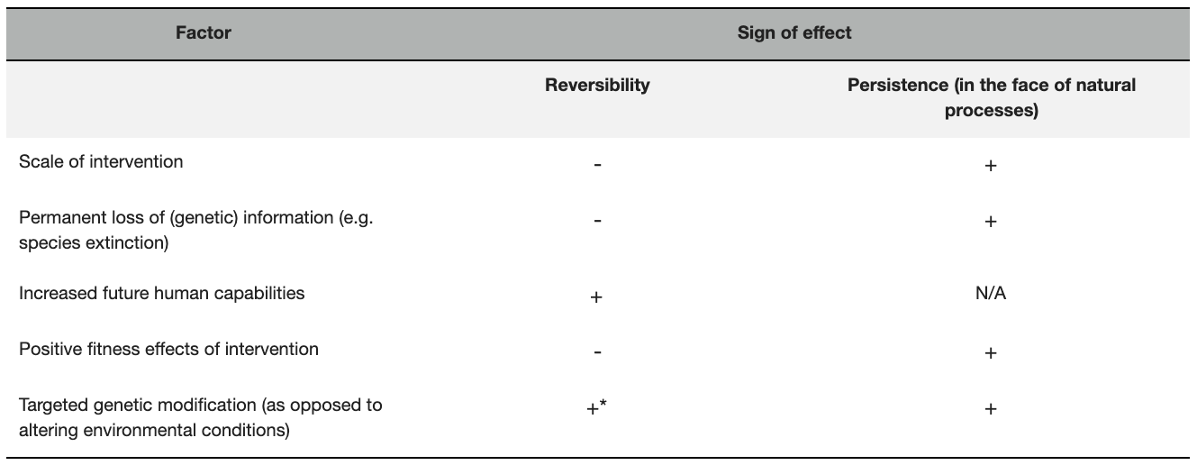 * If currently promising methods can be developed.
Will Bradshaw, Cameron Meyer Shorb, Lukas Finnveden, Jane Capozzelli, Kim Cuddington, Gustav Alexandrie, Michelle Graham, Abraham Rowe, Denis Drescher, and Luke Hecht have given very valuable feedback during the process of writing this report. This work was supported by the Effective Altruism Foundation.
Adger, W. N., Hughes, T. P., Folke, C., Carpenter, S. R., & Rockström, J. (2005). Social-ecological resilience to coastal disasters. Science, 309(5737), 1036-1039.
Anzalone, A. V., Randolph, P. B., Davis, J. R., Sousa, A. A., Koblan, L. W., Levy, J. M., ... & Liu, D. R. (2019). Search-and-replace genome editing without double-strand breaks or donor DNA. Nature.
Archer et al. (2009). Atmospheric lifetime of fossil fuel carbon dioxide. Annual review of earth and planetary sciences 37:117-134.
Askell, A. (2017). The moral value of information. https://www.effectivealtruism.org/articles/the-moral-value-of-information-amanda-askell/.
Barnosky, A. D., Matzke, N., Tomiya, S., Wogan, G. O., Swartz, B., Quental, T. B., ... & Mersey, B. (2011). Has the Earth’s sixth mass extinction already arrived?. Nature, 471(7336), 51.
Beckstead N. (2013). On the overwhelming importance of shaping the far future (Doctoral dissertation, Rutgers University-Graduate School-New Brunswick).
Beisner, B. E., Haydon, D. T., & Cuddington, K. (2003). Alternative stable states in ecology. Frontiers in Ecology and the Environment, 1(7), 376-382.
Bostrom N, & Ord T. (2006). The reversal test: eliminating status quo bias in applied ethics. Ethics, 116(4), 656-679.
Bostrom N. (2013). Existential risk prevention as global priority. Global Policy, 4:15-31.
Brennan, O. (2018). Wildlife Contraception. https://was-research.org/paper/wildlife-contraception/.
Brin, M., & Stuck, G. (2002). Introduction to dynamical systems. Cambridge university press. p. 25-27.
Burt, A. & Trivers, R. (2009). Genes in conflict: the biology of selfish genetic elements. Harvard University Press.
Collins J & Page L. (2019). The heritability of fertility makes world population stabilization unlikely in the foreseeable future. Evolution and Human Behavior, 40:105-111.
Cooney, C. R., Bright, J. A., Capp, E. J., Chira, A. M., Hughes, E. C., Moody, C. J., ... & Thomas, G. H. (2017). Mega-evolutionary dynamics of the adaptive radiation of birds. Nature, 542(7641), 344.
Curtis, R. J., Brereton, T. M., Dennis, R. L., Carbone, C., & Isaac, N. J. (2015). Butterfly abundance is determined by food availability and is mediated by species traits. Journal of Applied Ecology, 52(6), 1676-1684.
Cushing, J. M., Levarge, S., Chitnis, N., & Henson, S. M. (2004). Some discrete competition models and the competitive exclusion principle. Journal of Difference Equations and Applications, 10(13-15), 1139-1151.
Dempster, J. P., & Pollard, E. (1981). Fluctuations in resource availability and insect populations. Oecologia, 50(3), 412-416.
Dennis, B. (1989). Allee effects: population growth, critical density, and the chance of extinction. Natural Resource Modeling, 3(4), 481-538.
Dong, S. X., Davies, S. J., Ashton, P. S., Bunyavejchewin, S., Supardi, M. N., Kassim, A. R., ... & Moorcroft, P. R. (2012). Variability in solar radiation and temperature explains observed patterns and trends in tree growth rates across four tropical forests. Proceedings of the Royal Society B: Biological Sciences, 279(1744), 3923-3931.
Eskander, P. (2018a). To reduce wild animal suffering we need to find out if the cause area is tractable. https://animalcharityevaluators.org/blog/to-reduce-wild-animal-suffering-we-need-to-find-out-if-the-cause-area-is-tractable/.
Eskander, P. (2018b). An introduction to human appropriation of net primary productivity. https://was-research.org/paper/an-introduction-to-human-appropriation-of-net-primary-productivity/.
Esvelt, K. M., & Gemmell, N. J. (2017). Conservation demands safe gene drive. PLoS biology, 15(11), e2003850.
Esvelt, K. M., Smidler, A. L., Catteruccia, F., & Church, G. M. (2014). Emerging technology: concerning RNA-guided gene drives for the alteration of wild populations. Elife, 3, e03401.
Eurobarometer (2010). Biotechnology report. Bruxelles, Belgium: TNS Opinion and Social.
Fagan, W. F., & Holmes, E. E. (2006). Quantifying the extinction vortex. Ecology letters, 9(1), 51-60.
Fonseca, C. R., & Ganade, G. (2001). Species functional redundancy, random extinctions and the stability of ecosystems. Journal of Ecology, 89(1), 118-125.
Girardin, L., Calvez, V., & Débarre, F. (2019). Catch me if you can: a spatial model for a brake-driven gene drive reversal. Bulletin of mathematical biology, 81(12), 5054-5088.
Gotelli, N. J. (2001). A primer of ecology. Sunderland, MA: Sinauer Associates. (p. 112).
Graham, E. A., Mulkey, S. S., Kitajima, K., Phillips, N. G., & Wright, S. J. (2003). Cloud cover limits net CO2 uptake and growth of a rainforest tree during tropical rainy seasons. Proceedings of the National Academy of Sciences, 100(2), 572-576.
Grant, K. M., Rohling, E. J., Ramsey, C. B., Cheng, H., Edwards, R. L., Florindo, F., ... & Williams, F. (2014). Sea-level variability over five glacial cycles, Nat. Commun., 5, 5076.
Greaves H. (2017). Population axiology. Philosophy Compass, 12:e12442.
Greenwell, R. N., Ritchey, N. P., & Lial, M. L. (2003). Calculus with Applications for the Life Sciences—Markov Chains (online material). Boston: Addison Wesley.
Groff Z, & Ng YK. (2019). Does suffering dominate enjoyment in the animal kingdom? An update to welfare biology. Biology & Philosophy, 34:40.
Hastings, A., Abbott, K. C., Cuddington, K., Francis, T., Gellner, G., Lai, Y. C., ... & Zeeman, M. L. (2018). Transient phenomena in ecology. Science, 361(6406), eaat6412.
Hixon, M. A. (2008) Carrying capacity. In: Jorgensen, S.E., Fath, Brian. Encyclopedia of Ecology. London: Elsevier Science. p. 258-260.
Horta, O. (2010). Debunking the idyllic view of natural processes: Population dynamics and suffering in the wild. Télos, 17:73-88.
Huston, M. A., & Wolverton, S. (2009). The global distribution of net primary production: resolving the paradox. Ecological monographs, 79(3), 343-377.
IPCC. (2005). IPCC special report on carbon dioxide capture and storage. Prepared by working group III of the intergovernmental panel on climate change. Metz, B., O. Davidson, H. C. de Coninck, M. Loos, and L. A. Meyer (eds.). Cambridge University Press, Cambridge, United Kingdom and New York, NY, USA. (p 12).
Jensen, C. X., & Ginzburg, L. R. (2005). Paradoxes or theoretical failures? The jury is still out. Ecological Modelling, 188(1), 3-14.
Jinek, M., Chylinski, K., Fonfara, I., Hauer, M., Doudna, J. A., & Charpentier, E. (2012). A programmable dual-RNA–guided DNA endonuclease in adaptive bacterial immunity. science, 337(6096), 816-821.
Johannsen, K. (2017). Animal Rights and the Problem of r-Strategists. Ethical Theory and Moral Practice, 20(2), 333-345.
Keck, F. (2017) Changes in number of authors in ecology journals over time. http://www.pieceofk.fr/changes-in-number-of-authors-in-ecology-journals-over-time/.
Lindmark, R. (2018). Current Estimates for Likelihood of X-Risk? https://forum.effectivealtruism.org/posts/frYYAAa5K4nHqRCPG/current-estimates-for-likelihood-of-x-risk.
MacAskill, W. Manuscript a. Human extinction, asymmetry, and option value. https://docs.google.com/document/d/1hQI3otOAT39sonCHIM6B4na9BKeKjEl7wUKacgQ9qF8/. (p. 9).
MacAskill, W. Manuscript b. Should we expect moral convergence? https://docs.google.com/document/d/1EaIsqexbG2wiE7WIA_tyXiZjmbOmKc1Gy7rVQDSvMtg/.
Mahoney, J., & Schensul, D. (2006). Historical Context and Path Dependence. In Goodin, R., and Tilly, C., (eds.), The Oxford Handbook of Contextual Political Analysis. Oxford: Oxford University Press. Pp. 454-71.
Manthey M, Fridley JD and Peet RK (2011) Niche expansion after competitor extinction? A comparative assessment of habitat generalists and specialists in the tree floras of south‐eastern North America and south‐eastern Europe. Journal of Biogeography, 38:840-853.
Mathesius, S., Hofmann, M., Caldeira, K., & Schellnhuber, H. J. (2015). Long-term response of oceans to CO 2 removal from the atmosphere. Nature Climate Change, 5(12), 1107.
Matthews, D. (2018). A genetically modified organism could end malaria and save millions of lives — if we decide to use it. https://www.vox.com/science-and-health/2018/5/31/17344406/crispr-mosquito-malaria-gene-drive-editing-target-africa-regulation-gmo.
Min, J., Noble, C., Najjar, D., & Esvelt, K. (2017). Daisy quorum drives for the genetic restoration of wild populations. BioRxiv, 115618.
Nath S. (2016). The thermodynamic efficiency of ATP synthesis in oxidative phosphorylation. Biophysical chemistry, 219:69-74.
Nemani, R. R., Keeling, C. D., Hashimoto, H., Jolly, W. M., Piper, S. C., Tucker, C. J., ... & Running, S. W. (2003). Climate-driven increases in global terrestrial net primary production from 1982 to 1999. science, 300(5625), 1560-1563.
Noble, C., Min, J., Olejarz, J., Buchthal, J., Chavez, A., Smidler, A. L., ... & Esvelt, K. M. (2019). Daisy-chain gene drives for the alteration of local populations. Proceedings of the National Academy of Sciences, 116(17), 8275-8282.
Noble, C., Olejarz, J., Esvelt, K. M., Church, G. M., & Nowak, M. A. (2017). Evolutionary dynamics of CRISPR gene drives. Science advances, 3(4), e1601964.
O'Grady, J. J., Reed, D. H., Brook, B. W., & Frankham, R. (2004). What are the best correlates of predicted extinction risk? Biological Conservation, 118(4), 513-520.
Oye, K. A., Esvelt, K., Appleton, E., Catteruccia, F., Church, G., Kuiken, T., ... & Collins, J. P. (2014). Regulating gene drives. Science, 345(6197), 626-628.
Power M. (1992). Top‐down and bottom‐up forces in food webs: do plants have primacy. Ecology, 73:733-746.
Prevedello, J. A., Dickman, C. R., Vieira, M. V., & Vieira, E. M. (2013). Population responses of small mammals to food supply and predators: a global meta‐analysis. Journal of Animal Ecology, 82(5), 927-936.
Rakocevic, G., Djukic, T., Filipovic, N., & Milutinović, V. (2013). Computational medicine in data mining and modeling. New York: Springer. (p. 159).
Raup DM (1978) Cohort analysis of generic survivorship. Paleobiology, 4:1-15.
Raup D M (1991) A kill curve for Phanerozoic marine species. Paleobiology, 17:37-48.
Ray, G. (2017). Parasite load and disease in wild animals. https://was-research.org/paper/parasite-load-disease-wild-animals/.
Ricklefs R (2010) Evolutionary diversification, coevolution between populations and their antagonists, and the filling of niche space. Proc Natl Acad Sci USA 107:1265-1272.
Roser, M., and Ritchie, H. (2019) Technological Progress. https://ourworldindata.org/technological-progress.
Roser, M. (2019) Human Rights. https://ourworldindata.org/human-rights.
Ruffino, L., Salo, P., Koivisto, E., Banks, P. B., & Korpimäki, E. (2014). Reproductive responses of birds to experimental food supplementation: a meta-analysis. Frontiers in zoology, 11(1), 80.
Sandberg, A. & Bostrom, N. (2008): Global Catastrophic Risks Survey, Technical Report #2008-1, Future of Humanity Institute, Oxford University: pp. 1-5.
Shooster, J. (2017). Legal personhood and the positive rights of wild animals. https://was-research.org/writing-by-others/legal-personhood-positive-rights-wild-animals/.
Schubert, S., & Garfinkel, B. (2017). Hard-to-reverse decisions destroy option value. https://www.effectivealtruism.org/articles/hard-to-reverse-decisions-destroy-option-value/.
Singer, P. (1981). The expanding circle. Oxford: Clarendon Press.
Soberón J, Peterson AT (2005) Interpretation of models of fundamental ecological niches and species’ distributional areas. Biodiversity Informatics 2:1–10.
Solé, R. V., Ferrer‐Cancho, R., Montoya, J. M., & Valverde, S. (2002). Selection, tinkering, and emergence in complex networks. Complexity, 8(1), 20-33.
South, P. F., Cavanagh, A. P., Liu, H. W., & Ort, D. R. (2019). Synthetic glycolate metabolism pathways stimulate crop growth and productivity in the field. Science, 363(6422), eaat9077.
Steffen, W., Grinevald, J., Crutzen, P., & McNeill, J. (2011). The Anthropocene: conceptual and historical perspectives. Philosophical Transactions of the Royal Society A: Mathematical, Physical and Engineering Sciences, 369(1938), 842-867.
Stroud, J. T., & Losos, J. B. (2016). Ecological opportunity and adaptive radiation. Annual Review of Ecology, Evolution, and Systematics, 47.
Thomas, C. D. (2015). Rapid acceleration of plant speciation during the Anthropocene. Trends in Ecology & Evolution, 30(8), 448-455.
Todd, B. (2017). The case for reducing extinction risk. https://80000hours.org/articles/extinction-risk/.
Tomasik, B. (2016). Scenarios for very long-term impacts of climate change on wild-animal suffering. https://reducing-suffering.org/scenarios-for-very-long-term-impacts-of-climate-change-on-wild-animal-suffering/.
Tomasik, B. (2018a). Climate change and wild animals. https://reducing-suffering.org/climate-change-and-wild-animals/.
Tomasik, B. (2018b). Net primary productivity by land type. https://reducing-suffering.org/net-primary-productivity-land-type/.
Tyrrell T, Shepherd J, & Castle S. (2007). The long-term legacy of fossil fuels. Tellus B: Chemical and Physical Meteorology, 59:664-672.
Urban M. (2015). Accelerating extinction risk from climate change. Science, 348:571-573.
Valentine J. W. (1970) How many marine invertebrate fossil species? A new approximation. Journal of Paleontology, 410-415.
Vargas-Terán, M., Hofmann, H. C., & Tweddle, N. E. (2005). Impact of screwworm eradication programmes using the sterile insect technique. In Sterile insect technique (pp. 629-650). Springer, Dordrecht.
Warschefsky E, Penmetsa RV, Cook DR, & von Wettberg EJ. (2014). Back to the wilds: tapping evolutionary adaptations for resilient crops through systematic hybridization with crop wild relatives. American journal of botany, 101:1791-1800.
Webber, B. L., Raghu, S., & Edwards, O. R. (2015). Opinion: Is CRISPR-based gene drive a biocontrol silver bullet or global conservation threat?. Proceedings of the National Academy of Sciences, 112(34), 10565-10567.
The World Bank. (2016). Agricultural land (% of land area). http://data.worldbank.org/indicator/AG.LND.AGRI.ZS.
Wright, S. J., & Calderón, O. (2006). Seasonal, El Nino and longer term changes in flower and seed production in a moist tropical forest. Ecology letters, 9(1), 35-44.
When deciding whether to reverse an intervention, we want to use a utility function that assigns value to different states of the world (such as the world in which a bad intervention is reversed, and the world in which it is not). But, returning the world to the same physical state as it was before the intervention was implemented will not necessarily correspond to a maximization of utility. Even though a complete reversal of the world after a bad intervention would lead to a net gain in utility, there might be other states with higher utility, where the effect of the intervention can be said to be cancelled but the physical state of the world is not reversed.
Given the goal of maximizing welfare, then, assuming that we should always move back to the original state after an intervention goes poorly has similar qualities to the status quo bias (Bostrom & Ord 2006). The likelihood that the optimum configuration of the world just happens to match what we had before the intervention is fairly low (Bostrom & Ord 2006). This shortcoming of the concept of reversibility might not be a big problem, however. The ability to return the world to a state that contains the same moral value will likely correlate with how easily changes can be made to the state of the world (i.e. how malleable the system is). However, this proposed correlation is mainly conjecture and would need to be investigated further.
To conceptualize the measurement of the degree of reversal, we can consider the state of the world as a point in multidimensional state space, where every variable has its own axis and a point represents a complete description of the world in a given state. The difference between two states of the world is then measured as the euclidean distance between the worlds in state space. When assessing reversibility, we are thus measuring how much we can reduce the distance between the two worlds in state space.
An alternative approach, which is not considered in this report, is to measure the difference between worlds in a more granular way. We could for instance decide to only measure a subset of parameters, and then similarly calculate the euclidean distance between the worlds in this reduced state space. It is unclear if it is better to conceptualize reversibility as a complete or reduced state space, but a complete state space seems less arbitrary than choosing some parameters specific to each intervention and measuring reversibility only on those.
Lastly, it might be useful to distinguish between reversibility for different agents. It is possible that agents who care about wild animals, who might be in a minority even in the future, will have a reduced ability to affect states of natural systems, even if our aggregate capabilities would have increased. This could happen if one or a few agents or institutions have obtained a decisive strategic advantage, so as to largely exclude others from the decision-making processes.
Value of information (VOI) is a concept related to reversibility. The expected utility of future information about the effects of an intervention is affected by (1) the expected utility of a reversal given the information that the intervention produced a bad outcome, and (2) the probability of a bad outcome. The probability of a bad outcome is important, since it determines whether we can make use of the information by reversing the intervention. Thus, the VOI of intervention A is given by:
Box 3: Value of information
VOI = P_bad_outcome × EU_reversal

Where

VOI = value of information,

P_bad_outcome = probability of a bad outcome, and

EU_reversal = the maximum expected utility produced by a reversal (see equation 1 and Definition of reversibility for further detail)
Here we assume binary outcomes (not continuous probability distributions). The larger the probability of a bad outcome, and the larger the expected utility of reversing such an outcome by r is, the larger the value of information. Note that, for simplicity, we are substituting the extent to which we can move to the optimal state, with the extent to which we can move to the reversed state (see Reversibility as a proxy for malleability in Appendix A for a discussion about this). Furthermore, the expected utility of doing intervention A is defined as follows:
Box 4: Value of an intervention
EU_A = P_good_outcome × V_good_outcome − C_A × CE_intervention_B + P_bad_outcome × V_bad_outcome + P_bad_outcome × EU_rev

Where

EU_A = the expected utility of an intervention (intervention A),

V_good_outcome and V_bad_outcome = the utility that would be produced if there was a good or bad outcome, respectively,

P_good_outcome and P_bad_outcome = the probabilities of obtaining a good or bad outcome, respectively,

C_A = the cost of intervention A, and

EU_rev = the maximum expected utility produced by a reversal given a bad outcome
EU_A is the most decision relevant quantity of the ones discussed in this Appendix, since it gives you the expected utility of intervention A including the opportunity cost of not doing the next best thing (intervention B). If EU_A is positive, and given that we assume an expected utility approach, we should do intervention A.
See for instance: https://concepts.effectivealtruism.org/concepts/cost-effectiveness-analysis/. ↩︎
“Benefit” here refers to the benefit in expectation, which accounts for all possible outcomes (both positive and negative) in proportion to their likelihood. ↩︎
Note that the action could be any type of action, and does not necessarily have to be related to wild animal welfare. ↩︎
I assume here that continuing to reverse A is the action with the highest expected utility, as if it were not, you would just do whatever action has the highest expected utility. ↩︎
Relatedly, an alternative way of defining reversibility that applies in cases without diminishing returns of r to C_r, is the value of C_r when r = 1 (e.g. Schubert & Garfinkel 2017). ↩︎
Specifically, the product of C_r and CE_intervention_B gives this opportunity cost, in that it represents forsaken expected utility of intervention B given the total investment in reversing intervention A. ↩︎
The number of papers produced in ecology has been rising at a steadily increasing (perhaps exponential) rate since the 1950s (Keck 2017). ↩︎
Processor speed, memory storage, and many other aspects of computer efficiency have increased at roughly exponential speeds (Roser & Ritchie 2019). ↩︎
See the section A2 in the Appendix for a discussion of how the value of information relates to reversibility. See Askell (2017) for an explanation of how to estimate the value of information. ↩︎
Of course, one could define interventions maintained by humans as being persistent over time, but that type of pseudo-persistence is conditional on the continued upkeep and outlay of resources. The reason for restricting the definition of persistence is that independently persistent interventions have features that “maintained” interventions do not: they are likely to be more cost effective and less reversible. ↩︎
Although persistence can also be due to transient effects (Hastings et al. 2018), as an action that changes the state of a system can have effects that are long lasting even if the system moves (very) slowly back to the initial state through a transient state. Here, transient refers to the technical definition from Complexity Theory (Hastings et al. 2018). ↩︎
This is similar to how the resilience of states with regards to ecological systems is defined in Beisner et al. (2003), although they consider resilience to be a property of a system that can change over time, such that a system can be resilient currently but predictably non-resilient in the future. In this report, I take persistence to mean the expected (i.e. predicted) duration spent in a certain state, thus aggregating over all time slices. ↩︎
This assumes that the termination probability is constant over time, or that the strength/intensity of the effect of each intervention will exponentially decay. Other shapes of the survival function might apply, but without specific information about the shape of the distribution, we should opt for the maximum entropy distribution (the one with the fewest assumptions: Rakocevic et al. 2013, p. 159). In cases with non-negative values, such a distribution is described by an exponential decay function. ↩︎
Although if they are persistent because future humans approve of the intervention, we should not take credit for the full effect, since the counterfactual might have been that the intervention would have been implemented anyway. ↩︎
However, it is possible that such persistent interventions are more costly on average, at least in terms of research, than less persistent interventions. Intuitively it seems like making persistent changes to ecosystems is harder than making short-lasting changes, since evolutionary pressures and population dynamics often act as negative feedback loops to any fitness-decreasing changes. Furthermore, research into overcoming such negative feedback loops might be costly. These costs are probably not large enough to outweigh the added benefit of higher persistence. ↩︎
Assuming that there is some cost to restricting the space of possible interventions to reversible ones. ↩︎
For summaries of different estimates, see Todd (2017) and Lindmark (2018). ↩︎
For a similar discussion, see What is the likelihood of interventions being accepted and adopted? in Eskander (2018a). ↩︎
These selfish genetic elements copy themselves into the genomes of host organisms, with the capability of spreading among individuals within species, and even among species. The most common forms of naturally occurring gene drives are transposable elements, where multiple copies exist in the genome of most species (Burt & Trivers 2009, p. 228). ↩︎
An even newer and more precise gene editing technology, called prime editing, was recently described (Anzalone et al. 2019), which could replace CRISPR/Cas9 as the method of choice for gene drives. ↩︎
A gene is fixed within a population when all individuals share that particular gene variant. ↩︎
From a rights-based perspective, one might argue that modifying genes violates the autonomy of animals. However, many applications could plausibly be said to increase autonomy. For example, engineering disease resistance into animal populations would allow wild animals to live longer and fuller lives. For a broader discussion of rights-based perspectives on helping wild animals, see Shooster (2017). ↩︎
It might appear that an extinction is an infinitely stable change (to the extent that we cannot resurrect the species). However, this ignores the fact that the counterfactual is not that the species will exist forever; the average time until extinction for most animal taxa is a few million years (see Functional redundancy in ecosystems and niche expansion). ↩︎
The reason for gene drives being both persistent in the face of natural processes, and highly reversible, is probably related to the fact that the genetic code of living organisms has evolved to ‘defy’ entropy (by increasing entropy elsewhere) and retain information, while at the same time it has not evolved mechanisms to protect it against human gene modification tools. ↩︎
Underdominance is when heterozygotes (individuals with two different gene variants at a specific site) have lower fitness than homozygotes (individuals with the same gene variants at the specific site). ↩︎
A daisy drive is in many ways identical to a standard gene drive, but with a built in self-extinguishing effect (Noble et al. 2019). This is accomplished by having a series of genetic elements driving each other in a chain-like pattern, where the first link in the chain will be inherited as any other gene, and will thus be selected against. When the first link in the chain has been eliminated from the population, there is now nothing that is driving the second link, which will cause it to be purged from the population by natural selection. This continues until all gene drive elements have been eliminated. ↩︎
Another scenario that is conceivable based on the methods of Min et al. (2017), is speciation due to mate choice based on traits that might distinguish genetically modified individuals from wild type individuals. I find this implausible because such reproductive isolation would have to be established extremely fast. ↩︎
Extinction will here refer to the extinction of non-human animals. ↩︎
This is a bit of an illusory distinction, since most species will not survive in the absence of other organisms. It might be a useful heuristic though, especially in the case discussed here where perhaps just a single species is removed from the environment. ↩︎
“As in the case of range occupancy, however, species often are absent from locations that otherwise are judged to be appropriate” (Ricklefs 2010, pages 84–86). ↩︎
It would be interesting to see empirical or theoretical work quantifying the difference between the fundamental and realized niche, and the effects of species removal on niche occupancy, ideally with a focus on the welfare of the extinct and the replacing species. Studies such as the study by Manthey et al. (2011), looking at the difference between the fundamental niche and the realized niche, would be needed to get estimates of the time to niche replacement. Furthermore, studies on the speed of evolution of phenotypic character displacement might give indications of how quickly certain characters can re-evolve once the displacement pressure disappears. ↩︎
The mean duration of invertebrate genera in the fossil record during the Phanerozoic Eon (i.e. from the Cambrian period, 541 million years ago, until present) is 11.1 million years (Raup 1978). According to a review of the literature by Valentine (1970), the mean duration of marine invertebrates is somewhere between 5 and 10 million years. Raup (1991) followed up his previous study on invertebrates (Raup 1978), but focused specifically on marine animals (including marine vertebrates as well), and found that the average duration of genera was 4 million years. However, he seemed to think differences in the results (11.1 and 4 million years) were due to differences in statistical methods rather than differences in the underlying data. If this is correct, the results of Raup (1991) are likely more accurate, since that estimate was produced later. It should be noted that the genus is commonly used as opposed to species when calculating extinction rates (e.g. Raup 1978, 1991), but the most relevant level for the discussion of gene drives is the species level. ↩︎
This has been written about previously (long-term effects: Tomasik 2016; and short-term effects: Tomasik 2018a). ↩︎
This is due to the difficulty of predicting the welfare implications of for instance distribution and population size changes of wild animals. ↩︎
Even if the effects of climate change would be positive for wild animal welfare, it does not follow that we should not try to mitigate the effects of climate change. From a longtermist perspective (Beckstead 2013; Bostrom 2013), actively increasing the risk of human extinction brought about by extreme climate change could be very bad (assuming that the expected utility of humanity’s continued existence is positive). ↩︎
Although earlier studies have produced estimates that differ substantially from Archer et al. (2009) and each other (see table 1 in Tyrrell et al. 2007). ↩︎
"In most scenarios for stabilization of atmospheric greenhouse gas concentrations between 450 and 750 ppmv CO2 and in a least-cost portfolio of mitigation options, the economic potential of CCS would amount to 220–2,200 GtCO2 (60–600 GtC) cumulatively, which would mean that CCS contributes 15–55% to the cumulative mitigation effort worldwide until 2100, averaged over a range of baseline scenarios." (IPCC 2005, p. 12). ↩︎
It is also possible that energy efficiency enhancements could be carried out directly on animals, although I think it is fairly unlikely. The efficiency of cellular respiration in animals seem to be around 40% (Nath 2016), which indicates that there is room for efficiency improvements at the biochemical level, at least in principle. ↩︎
For a summary, see: https://ripe.illinois.edu/objectives/photorespiratory-bypass. ↩︎
For tentative discussions on the effects of changes in net primary productivity (NPP) on wild animal welfare, see Tomasik (2018b) and Eskander (2018b). ↩︎
There are indirect measures suggesting a relationship between primary productivity and animal biomass (Huston & Wolverton 2009), which probably partly manifests as an increase in the total number of individual animals. By definition, with zero primary production by plants and other organisms, no heterotrophic organisms (i.e. organisms that cannot produce their own food) can be sustained. Consequently, there is definitely a positive relationship between the total number of individual animals and primary production, at least for the lower part of the primary production range. ↩︎
Humans are probably an exception, although similar processes might affect us as well in the future (Collins & Page 2019). ↩︎
These time scales are in the order of 0.1 to 10 speciation events per million species years (Thomas 2015). ↩︎