Ambiguity aversion and
reduction of X-risks: A
modelling situation

Benedikt Schmidt

Ambiguity aversion is a preference for known over unknown risks and influences decision-making. Ambiguity (also uncertainty) is particularly prevalent in the study of existential risk and is a diverse phenomenon. The following post analyses the influence of ambiguity aversion by means of the -maxmin model in a specific choice situation: Should an individual put their efforts in some proximate altruistic projects (PAP) or in the more long-term reduction of X-risks (RXR)?

Theoretical framework

Decision modelling

A choice situation is described by four basic structures (Etner 2012): The state space endowed with a -algebra A choice situation is described by four basic structures (Etner 2012): The state space $S$ endowed with a $σ$ -algebra $Σ$ of events (Stoye 2011), the outcome space $O$ , a set $A$ of mappings $f : S \to O$ and a preference relation $≿$ , which is defined over the mappings from $S$ to $O$ .
The expected utility (Chandler 2017) of an act is a weighted average of the utilities of each of its possible outcomes.

E U (f) = \sum o \in O P_{f} (o) u (o)

Different types of uncertainty

One can distinguish two fundamental origins of uncertainty (Bradley 2017):

uncertainty from features of the world like indeterminacy or randomness (objective uncertainty)
uncertainty from lack of information about the world (subjective or epistemic uncertainty)

Epistemic uncertainty can be further split into several subtypes:

Type of uncertainty	associated question
empirical/factual	What is the case?
evaluative	What should be the case?
modal	What could be the case?
option	what would be the case if we were to make an intervention of some kind?
Types of uncertainty

Ambiguity Aversion

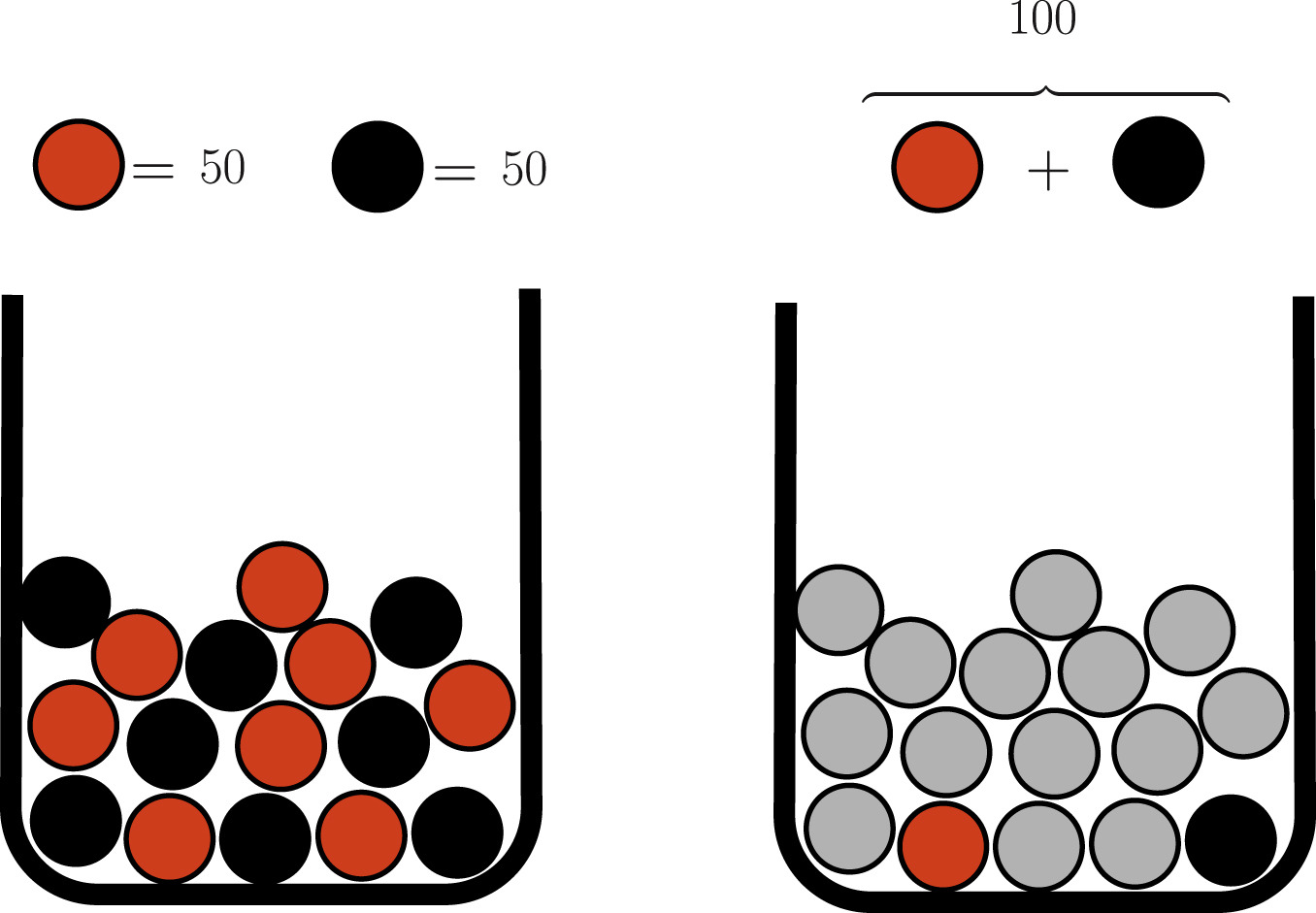
If it is possible to assign probabilities to the uncertainties in question, the situation is called risky. If the assignment of an objective probability is not possible, the situation is ambiguous. Ambiguity aversion is an aversion against ambiguous situations, first described by Ellsberg (Ellsberg 1961). Ambiguity averse agents prefer the urn on the left in Fig. 1.

Fig. 1: Ellsberg two-color problem (Eichenberger and Pirner 2018)

Modelling ambiguity aversion

In the $α$ -maxmin expected utility model (Ghirardato et al. 2004) an act $f \in A$ is evaluated in terms of expected utility:

E U (f) = α min p \in C E_{p} U (f) + (1 - α) max p \in C E_{p} U (f)

$α \in (0, 1]$ is a uniquely defined coefficient and an index of ambiguity aversion. $C$ is a set of priors (credal set).

Modelling situation

In order to analyze the influence of ambiguity aversion, following Mogensen 2018, consider an altruistic person (decision maker) facing the decision whether to put his efforts in the long-term reduction of X-risks (RXR) or in proximate altruistic projects (PAP). Hence we consider the two acts RXR and PAP. We want to look at the impact of the person under different circumstances. There are two ways the person could fail having any impact at all, namely if their effort is not necessary or if their effort is not sufficient for the achievement of the targeted effects.

Two extreme cases

Based on these two modes of failure and , we will consider two different cases:

Case 1: RXR is assumed to be sufficient to prevent EC (existential catastrophe), but perhaps unnecessary. If the decision maker chooses RXR, the future will be good for sure.
Case 2: RXR is assumed to be necessary to prevent EC, but perhaps insufficient. If the decision maker chooses PAP instead of RXR, EC will happen for sure.

For both cases, the impact shall be specified in agent-neutral value. Besides, consider two probabilistic criteria: Whether or not RXR prevents EC. Then we can set up two decision matrices:

	RXR prevents EC	RXR does not prevent EC
	$p_{x} \in [0, 0.02]$	$(1 - p_{x}) \in [0.98, 1]$
PAP	1	101
RXR	100	100
Case 1

An ambiguity-averse decision maker goes for RXR, because there, an expected value of 100 is guaranteed.

	RXR prevents EC	RXR does not prevent EC
	$p_{x} \in [0, 0.02]$	$(1 - p_{x}) \in [0.98, 1]$
PAP	1	1
RXR	100	0
Case 2

In Case 2, an ambiguity averse agent will opt for PAP, because, in contrast to RXR, it does not involve ambiguity (PAP yields for sure an agent-neutral value of 1).

Generalization

In order to generalize beyond the two extreme cases, we will still follow the structure of necessity and sufficiency. Consider the act RXR for prevention of EC. It can be unnecessary, then we don`t care about sufficiency. It can bu necessary but insufficient or both necessary and sufficient. With those 3 possibilities we can set up a generalized decision matrix where the agent-neutral value is denoted by variables:

	EC independent of choice	splendid future if RXR is chosen, EC otherwise	splendid future independent of choice
	$1 - P_{1} - P_{2}$	$P_{1}$	$P_{2}$
PAP	$y$	$y$	$w$
RXR	$z$	$x$	$x$
Generalized decision matrix

The worst case is represented by $z$ , where the agent neither enjoys the benefits of PAP, nor those of RXR. $y$ represents the value yielded by the choice of PAP whereas $x$ corresponds to the value yielded by the choice of RXR. The best case arises if the agent chooses PAP while RXR is not necessary, since then the agent-neutral value incorporates the benefits of PAP and RXR, amounting to $w$ . Therefore, clearly the following relation holds:

w > x > y > z

From the definition of the four variables, the following equivalence can be deduced:

w - y = x - z ⟺ w - x = y - z

This seems reasonable, since the value achieved through PAP is independent of whether humanity goes extinct later or not. Since we are interested in the relation between the benefits of PAP and RXR, we define the quotient $β$ as

β := \frac{y - z}{x - z} = \frac{w - x}{x - z}

$β$ thus represent the ratio of the respective values achieved by PAP and RXR. Since $y < x$ and also $z < y$ , it holds that $0 < β < 1$ .

The analysis yielded the following conditions: An ambiguity averse agent favors RXR over PAP if $E U (R X R) > y - z$ , i.e. if

α (min P \in C P - min P_{2} \in C_{2} P_{2}) + (1 - α) (max P \in C P - max P_{2} \in C_{2} P_{2}) > β

The same agent favors PAP over RXR if the converse inequality holds, i.e. if

α (min P \in C P - min P_{2} \in C_{2} P_{2}) + (1 - α) (max P \in C P - max P_{2} \in C_{2} P_{2}) < β

Discussion

We found that the choice of an ambiguity averse agent differs between the two cases considered: In Case 1a, where RXR is known to be sufficient, ambiguity aversion seems to favour RXR. In contrast, in Case 2a, where RXR is known to be necessary, ambiguity aversion favours PAP. This difference shows that the decision varies according to the setting. In reality, we are of course never sure that RXR will be sufficient. Rather, we can be sure that certain interventions decrease particular risks. It seems more plausible that we can be sure about the necessity of certain interventions. In this case, ambiguity aversion pushes the decision maker towards PAP. Then ambiguity aversion would not be helpful for the mitigation of X-risks.

Conclusion

Through decision theoretic analysis of our modelling situation, we specified conditions under which ambiguity aversion plays in favour for RXR and conditions, under which it pushes the decision maker towards PAP. In the study of X-risks, there are always different types of uncertainty involved. Almost never are we able to assign precise probabilities. Nevertheless, the decision theoretic approach presented here builds heavily on probabilities. This is because such an approach is helpful as a structure for our thinking. It can guide us through different aspects of the situation at hand. Besides, a formal approach allows to standardize to a certain extent. The latter is important since it is a condition for arriving at general statements. We did several assumptions in order to simplify the modelling situation. Even if those simplifications weaken the expressiveness of the results, they nevertheless are justified by the complexity of the issues under investigation. A theoretically more sophisticated analysis, which was not in the scope of this project, could maybe integrate more aspects and analytical tools.

Acknowledgements

This post is based on my research project in the Swiss Existential Risk Initiative. Views and mistakes are my own.

References

Etner, Johanna, Meglena Jeleva, and Jean-Marc Tallon (Apr. 2012). “DE-
CISION THEORY UNDER AMBIGUITY: DECISION THEORY UN-
DER AMBIGUITY”. In: Journal of Economic Surveys 26.2, pp. 234–
270. http://doi.wiley.com/10.1111/j.1467-6419.2010.00641.x (visited
on 07/02/2021).

Bradley, Richard (2017). Decision theory with a human face. OCLC: 1015858884.
Cambridge: Cambridge University Press. isbn : 978-1-108-54787-1 978-0-
511-76010-5. https://doi.org/10.1017/9780511760105 (visited
on 07/02/2021).

Chandler, Jake (2017). “Descriptive Decision Theory”. In: The Stanford En-
cyclopedia of Philosophy. Ed. by Edward N. Zalta. Winter 2017. Meta-
physics Research Lab, Stanford University.

Eichberger, Jürgen and Hans Jürgen Pirner (Oct. 2018). “Decision theory
with a state of mind represented by an element of a Hilbert space: The
Ellsberg paradox”. In: Journal of Mathematical Economics 78, pp. 131–
141. https://linkinghub.elsevier.com/retrieve/pii/S0304406818300193
(visited on 08/17/2021).

Ellsberg, Daniel (Nov. 1961). “Risk, Ambiguity, and the Savage Axioms”. In:
The Quarterly Journal of Economics 75.4, p. 643. https://academic.oup.com/qje/article-
lookup/doi/10.2307/1884324 (visited on 07/30/2021).

Ghirardato, Paolo, Fabio Maccheroni, and Massimo Marinacci (Oct. 2004).
“Diﬀerentiating ambiguity and ambiguity attitude”. In: Journal of Eco-
nomic Theory 118.2, pp. 133–173. https://linkinghub.elsevier.com/retrieve/
pii/S0022053104000262 (visited on 07/28/2021).

Mogensen, Andreas L. (2018). “Long-termism for risk averse altruists”. Un-
published Manuscript.

Stoye, Jörg (Feb. 2011). “Statistical decisions under ambiguity”. In: Theory
and Decision 70.2, pp. 129–148. http://link.springer.com/10.
1007/s11238-010-9227-2 (visited on 07/02/2021).

Gordon Seidoh WorleySep 13 20214

I didn't quite follow. What's the reasoning for claiming this?

Benedikt SchmidtSep 15 20212

The reasoning is the following:

The agent-neutral values are now denoted by variables instead of numbers.
The worst case is represented by , where the agent neither enjoys the beneﬁts
of PAP, nor those of RXR. $y$ represents the value yielded by the choice of
PAP whereas $x$ corresponds to the value yielded by the choice of RXR. The
best case arises if the agent chooses PAP while RXR is not necessary, since
then the agent-neutral value incorporates the beneﬁts of PAP and RXR,
amounting to $w$ . Therefore, clearly the following relation holds:

w > x > y > z

From there, the equivalence under question follows.

Do you agree?

Gordon Seidoh WorleySep 16 20212

I guess I don't understand why w > x > y > z implies w - y = x - y iff w - x = y - z. Sorry if this is a standard result I've forgotten, but at first glance it's not totally obvious to me.

Benedikt SchmidtSep 16 20211

Maybe it gets clearer if you compare the relative values of the 4 variables. corresponds to the benfits of RXR, $x - z$ also corresponds to the benefits of RXR. But maybe I was not precise enough: The equivalence does not follow only from $w > x > y > z$ , we also need to take into account the definitions of the 4 variables.
Do you see what I mean?

Venky1024Sep 14 20211

I didn't get the intuition behind the initial formulation:

What exactly is that supposed to represent? And what was the basis for assigning numbers to the contingency matrix in the two example cases you've considered?

Benedikt SchmidtSep 15 20213

Thanks for your question!
This is how the -maxmin model is defined. You can consider the coefficient $α$ as a sort of pessimism index. For details, see the source Ghirardato et al.

It is supposed to represent the extreme cases.
The numbers in the examples are exemplary. The purpose is to have two different cases in order to study.

Effective Altruism Forum
EA Forum

Ambiguity aversion and reduction of X-risks: A modelling situation

29