You can get a sense for these sorts of numbers just by looking at a binomial distribution.
e.g., Suppose that there are n events which each independently have a 45% chance of happening, and a noisy/biased/inaccurate forecaster assigns 55% to each of them.
Then the noisy forecaster will look more accurate than an accurate forecaster (who always says 45%) if >50% of the events happen, and you can use the binomial distribution to see how likely that is to happen for different values of n. For example, according to this binomial calculator, with n=51 there is a 24% chance that at least 26/51 of the p=.45 events will resolve as True, and with n=201 there is a 8% chance (I'm picking odd numbers for n so that there aren't ties).
With slightly more complicated math you can look at statistical significance, and you can repeat for values other than trueprob=45% & forecast=55%.
Great work and great writing, thank you. I wonder if there's anything better powered than t-tests in this setting though?
ETA: is "which forecaster is best?" actually the right question to be answering? If the forecasts are close enough that we can't tell the difference after 100 questions, maybe we don't care about the difference?
Can't think of anything better than a t-test, but open for suggestions.
If a forecaster is consistently off by like 10 percentage points - I think that is a difference that matters. But even in that extreme scenario where the (simulated) difference between two forecasters is in fact quite large, we have a hard time picking that up using standard significance tests.
Intuitively, I think there should be a way to take advantage of the fact that the outcomes are heavily structured. You have predictions on the same questions and they have a binary outcome.
OTOH, if in 20% of cases the worse forecaster is better on average, that suggests that there is just a hard bound on how much we can get.
If I can modus tolens this modus polens, it feels to me that
Indeed, even for 100 questions [...] this would come up as significant less than 50% of the time
is evidence that the noise level is low, and the skill difference is small.
E.g., taking the top 20 forecasters in Metaculus' last Quarterly Cup, we see average score differences of ~0.05 (equivalent to your highest noise level), and that's among the very top forecasters we had on that tournament!
Note: This is a linkpost for the Metaculus Journal. I work for Metaculus and this is part of a broader exploration of how we can compare forecasting performance.
Introduction
"Which one of two forecasters is the better one?" is a question of great importance. Countless internet points and hard-earned bragging rights are at stake. But it is also a question of great practical concern to decision makers. Imagine you are king Odysseus of Ithaca and you urgently need counsel for important government affairs. You vividly remember the last time you went away on a journey and now ask yourself: Is Delphi really worth the extra mile, or is the oracle of Dodona just as good?
Being Odysseus, a man of cunning, you quickly think of ways to obtain more knowledge. The obvious answer, of course, would be to run a forecasting tournament between the two oracles. But how many forecasting questions do you need? Divine revelations are expensive. And once the questions resolve and one oracle comes out ahead, how sure can you be that the winning oracle is really better? Oracling is not an exact science and sometimes, after all, the gods do play dice. Even a perfect oracle (who always reports a probability equal to the true probability of an event) will sometimes look bad if Tyche is not on her side.
Methods
You quickly decide you need to run a simulation study. That way you will know the 'true probabilities' of events. You can easily compare a perfect forecaster with a noisy forecaster and see whether the difference comes out as significant. You want to look at binary outcomes, meaning that either an event happens (outcome = 1) or it doesn't (outcome = 0). You also decide to restrict the analysis to only two forecasters to avoid issues with multiple comparisons and additional complications. Battles become complicated if too many factions are involved.
You choose to do a thousand replications of your experiment. For every replication, you simulate 1000 true probabilities, observations and corresponding forecasts. You then add increasing amounts of noise to the forecasts, score them, and then do a paired t-test to check whether there would be a significant difference between a noisy forecaster and a perfect forecaster.
There is a qualitative difference between a forecast that is moved from 50% to 55% and one that is moved from 94.5% to 99.5%. The former is only a small update, whereas the latter corresponds to a massive increase in confidence. This becomes obvious when you convert the probabilities to odds (odds = p / (1 - p)). The move from 50% to 55% would mean a move from 10:10 to 11:9 expressed as odds. the move from 94.5% to 99.5% would mean a move from 189:11 to 1990:10. To reflect this, you decide to convert your probabilities to log odds, add some normally distributed noise, and convert back to probabilities:
(You could of course also multiply odds by some noise instead of adding noise to log odds, but the latter is more elegant and computationally efficient. You are, after all, Odysseus the Cunning, and don't care about the fact that logarithms were first described - invented? - in 1614).
This is the precise algorithm you use:
For each of 1000 replications:
1. Draw N = 1000 true probabilities as a random uniform variable between 0 and 1
2. Create N = 1000 observations as draws from a Bernoulli distribution (drawing either a 0 or a 1) with the probability of drawing a 1 equal to the true probabilities drawn in step 1)
3. Create 5 forecasts from with differing noise levels, 0 (no noise), 0.1, 0.3, 0.5, and 1
- Convert probabilities to log odds (log (p / 1-p))
- noisy_log_odds = log_odds + N(mean = 0, sd = noise level)
- Convert back to obtain noisy probabilities
4. Score the forecasts using the log score
- For different noise levels and number of observations
5. Use a paired t-test to check whether the difference in score between the noisy forecaster and the perfect forecaster (no noise) is significantly different from zero
The log score is a proper scoring rule, meaning that it can't be cheated and forecasters are always incentivised to report their true belief. It is commonly defined as the negative logarithm of the forecast probability evaluated at the observed outcome. If your forecast is p that an event will actually happen and it happens (outcome = 1), then your log score is −logp. If it does not happen (outcome = 0), then your log score is −log(1−p). Smaller values are good (best is 0) and larger values are bad (the log score represents a penalty).
Results
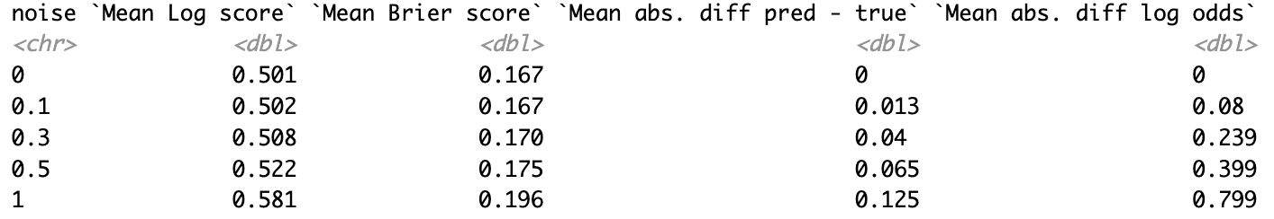
Here is a summary of the simulated data. The perfect forecaster (no noise) gets a log score of 0.501, the noisiest one a log score of 0.581. The next column shows the mean absolute difference between a forecaster's predictions and the true probability. This is 0 for the perfect forecaster (who always reports the true probabilities). For the forecaster with noise level 0.5, for example, their prediction on average differs by 6.5 percentage points from the perfect forecaster. The last column shows the difference between perfect forecast and noisy forecast in log odds space. The table shows Brier scores as well as those are more intuitive for some readers.
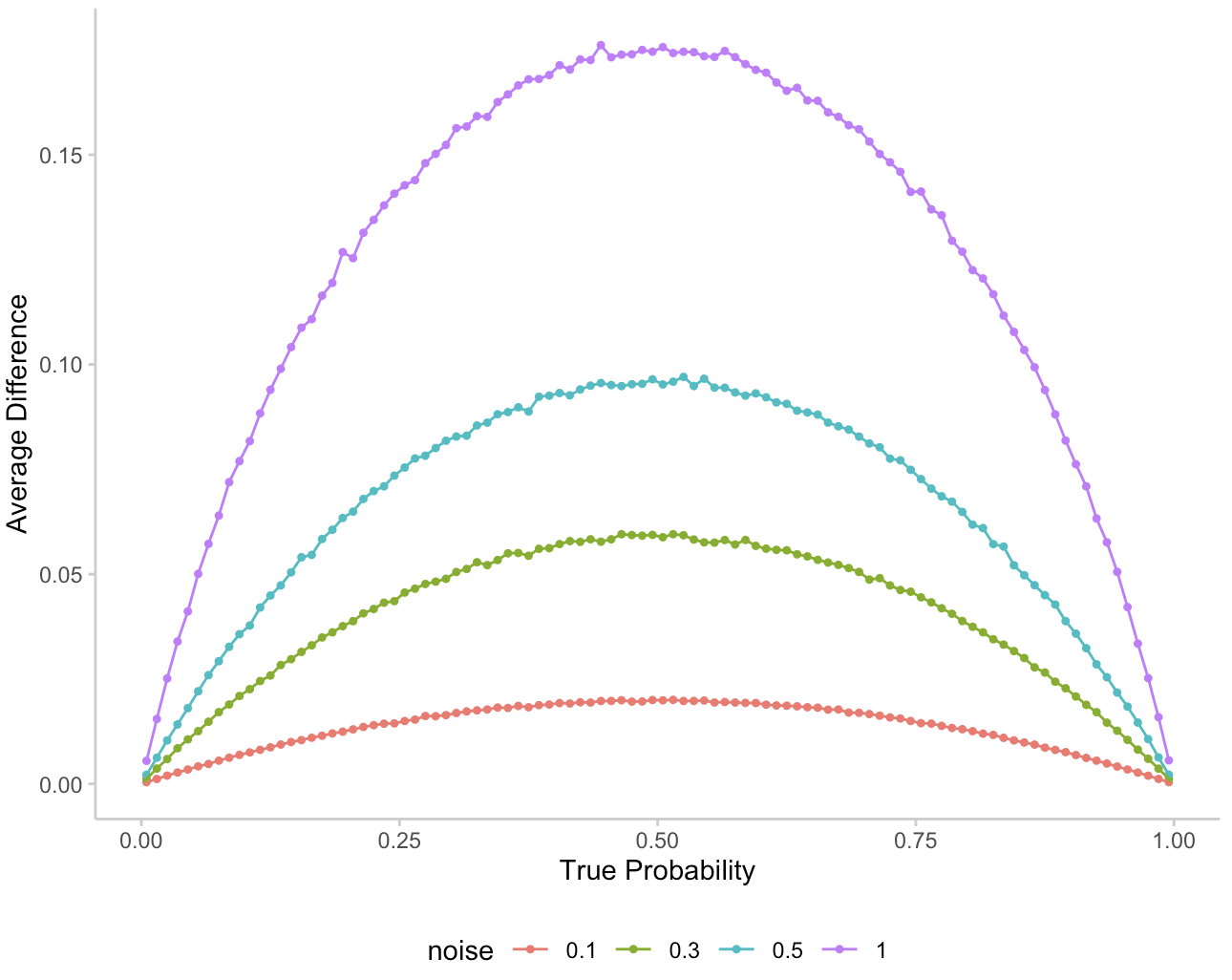
Given the way the noise was constructed, the average absolute difference between prediction and true probability is slightly deceiving. Adding noise in log odds space leads to probability differences that appear higher in absolute terms when predictions are closer to 0.5. This is illustrated in the following plot:
Figure 1: Average difference between the probability prediction of the noisy forecaster and the true probability.
Delphi or Dodona - significant choices
Now, how easy is it in an ideal world to say that one forecaster is significantly better than another? You, Odysseus the Cunning, predate the invention of the t-test by around 3 thousand years. But that shall not prevent you from applying a paired t-test to compare your noisy forecasters against the perfect forecaster. To simulate the effect of the number of available questions on the significance level, you run your tests for a different number of questions included. Here are your results:
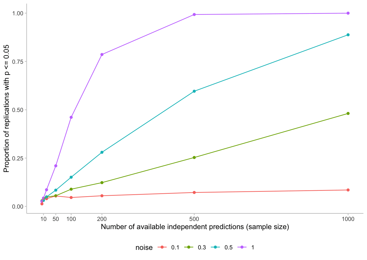
Figure 2: The proportion of replications in which forecasts from the perfect forecaster are deemed to be significantly better than those of the noisy forecaster
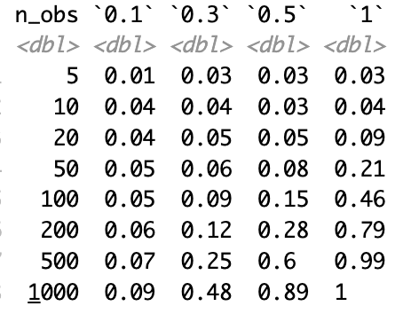
The plot shows the proportion of replications that bring up a significant difference between a noisy forecaster and the perfect forecaster. The following shows the same information as a table:
You scratch your head and beard in astonishment. "By Zeus! It seems like even in an ideal world I need quite a few observations (or quite a large difference in skill) to validly conclude that two forecasters are significantly different".
Indeed, even for 100 questions (which is rather large for a typical forecasting tournament) and a fairly large difference in forecaster performance, this would come up as significant less than 50% of the time. And in an actual real life forecasting tournament, we couldn't even be sure that the questions are completely uncorrelated. If they are, then that reduces the effective sample size and you'd need even more observations.
But would the better forecaster at least win in a direct stand-off? Would the perfect forecaster have a lower average log score than the noisy one? You go back to your abacus and move a few marbles to crunch the numbers again. This is your result:
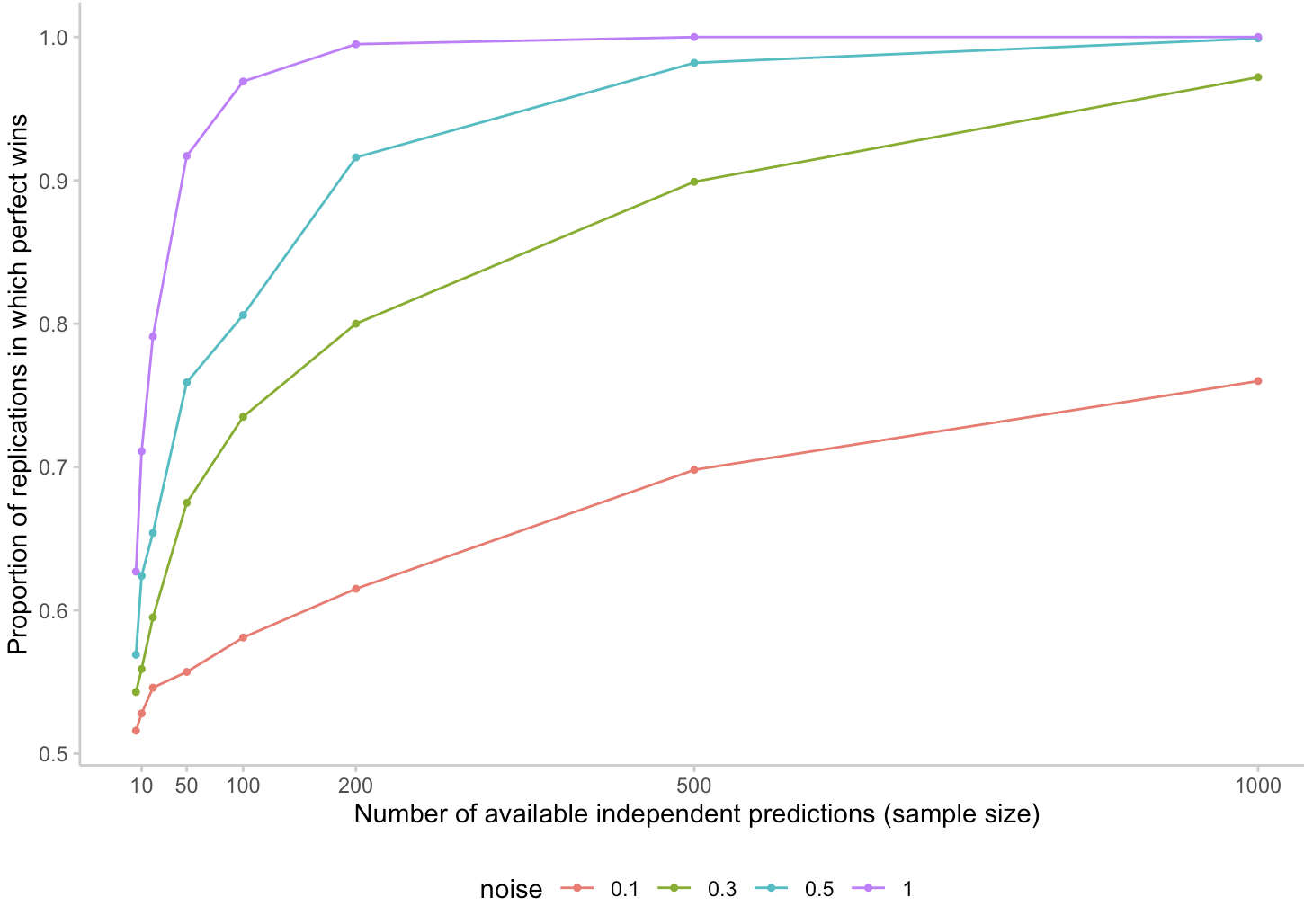
Figure 3: The proportion of replications in which the perfect forecaster beats the noisy forecaster, i.e. has a lower mean log score across all available questions
You take a deep breath. This also doesn't look ideal. The noisiest forecaster would win against the perfect forecaster around 8% of the time in a tournament with 50 questions. But a forecaster who is just half as noisy would already win about 24% of the time in the same tournament. That's still assuming that all questions are perfectly independent. You try to console yourself: The fact that the perfect forecaster would win against the noisiest forecaster in a 50 question tournament 92% of the time isn't too bad! But then you sigh: "Not too bad, but still useless. This info would make me happy if I were a (perfect) forecaster! But sadly I'm just a poor king in Ithaca and I still don't know which oracle to trust."
Conclusions
Decision makers want to know if one forecaster is better than the other. This is the one they should listen to. The last simulation (Figure 3) suggests that a noticeably better forecaster has a decent chance of winning a direct comparison. The problem is that even if both forecasters are equally good, one of them has to win. The mere fact that one of them won is some evidence they are better, but not that much. Even with a quite noticeable difference in performance and in an ideal scenario, it takes quite a few questions to make a decision at a standard 5%-significance level. This is important to know, and we should adjust our expectations accordingly whenever we try to compare between two forecasters, forecasting platforms, or oracles.
You, Odysseus, sit down on a rock. "How, by Zeus, am I supposed to run 500 questions by the oracles of Dodona and Delphi? Get their answers and wait for all the questions to resolve? This is nothing a mere mortal can do! I really wish all major oracles would just share their questions among each other. Every oracle could make predictions on all of them and over time we would have a great database with all their track records." You look up to the skies and send a short prayer to the holy quintinity of Metaculus, INFER, Good Judgment, Hypermind, and Manifold. "This would indeed be a project worthy of the gods!"
This is the third in a sequence of posts taken from my recent report: Why Did Environmentalism Become Partisan?
Summary
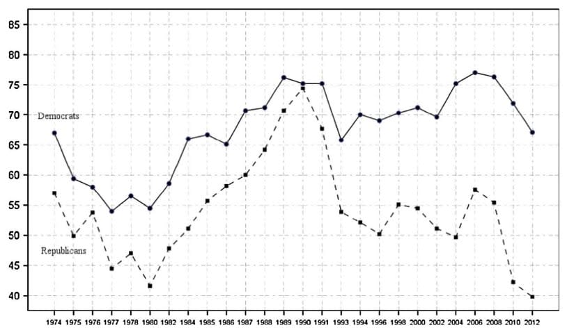
Rising partisanship did not make environmentalism more popular or politically effective. Instead, it saw flat or falling overall public opinion, fewer major legislative achievements, and fluctuating executive actions.
Public Opinion...
This post presents the executive summary from Giving What We Can’s impact evaluation for 2025. At the end of this post we share links to more information, including the full report and...

You can get a sense for these sorts of numbers just by looking at a binomial distribution.
e.g., Suppose that there are n events which each independently have a 45% chance of happening, and a noisy/biased/inaccurate forecaster assigns 55% to each of them.
Then the noisy forecaster will look more accurate than an accurate forecaster (who always says 45%) if >50% of the events happen, and you can use the binomial distribution to see how likely that is to happen for different values of n. For example, according to this binomial calculator, with n=51 there is a 24% chance that at least 26/51 of the p=.45 events will resolve as True, and with n=201 there is a 8% chance (I'm picking odd numbers for n so that there aren't ties).
With slightly more complicated math you can look at statistical significance, and you can repeat for values other than trueprob=45% & forecast=55%.
Good comment, thank you!