Here is one speculation of what could explain the prevalence of heavy-tailed distributions in what you call 'hierarchical classification schemes':
Suppose that the causal mechanism generating the relevant classes has the property that new members are more likely to be added to a class the more members it already has (e.g. if people were more likely to move to a city the higher its population). Under some such conditions it's then a mathematical consequence that the size distribution (i.e. number of members across classes) will converge to a power law.
This has been popularized as "preferential attachment" by the 'network science' people around Barabasi since the end of the 1990s to explain various observations on the Internet and other networks (though the related academic cottage industry has recently received some good criticism). But the maths and potential real-world cases are much older; indeed, the perhaps first major case for which this explanation was proposed was one of your examples - biological taxa -, by Yule in the 1920s.
You point to skewness as the key mathematical concept. However, I think that most of what you discuss (e.g. "outliers which drive up the mean") is better captured by kurtosis or other measures of 'heavy-tailedness' (and sometimes we may care more about the more familiar concept of variance).
In practice these will often be similar, so whether we look for e.g. "highly skewed" or "heavy-tailed" distributions often won't make a difference.
However, conceptually they are quite different. Skewness is related to the third central moment, i.e. the third power of deviations from the mean. This means it largely measures whether we have more outliers toward the right or toward the left of the mean, and thus is a measure of 'asymmetry'.
But arguably we often care more about how much weight outliers in either direction have compared to 'typical' values, or by how much future outliers might exceed the maximum value we've seen so far. I.e. 'absolute' measures of heavy-tailedness that are not defined by way of comparison to the tail on the other end of the distribution. Then we may be more interested in a measure of heavy-tailedness that is applied to just one tail of the distribution; or in kurtosis, which is related to the fourth central moment, i.e. the fourth square of deviations from the mean and thus a measure of how much weight outliers on either side have compared to typical values.
Concretely, skewness can be unintuitive for distributions that are multimodal (which can drive up skewness for a quite different reason than the distribution having a heavy or long tail on one side), or for distributions that have heavy/long tails on both sides but to different degrees.
Thanks for this post, I'm glad to see more attention on what I believe is an important topics (see also here).
I'm actually about to publish a related piece I wrote with Ben Todd specifically on whether the distribution of impact-related metrics across people is heavy-tailed. So this post is a nice complement. I particularly appreciate the specific data sets you point to.
For now I'm just going to make a couple of quick points, split between comments to allow for a more organized discussion.
--
One thing I would highly encourage you to do if you haven't already is to take a look at Power-law distributions in empirical data by Clauset et al. In particular, as explained in this paper:
I'm not sure what exactly you did when saying "The (least-squares estimate of the) power parameter p equals 0,6 for the education interventions, 1,02 for the health interventions and 1,8 for the climate policies.", but note that one needs to be careful here. In particular, doing a standard linear regression / least-squares fit in a log-log plot is generally not a valid way of estimating the power law parameters. You need to use something like maximum likelihood estimation.
More broadly, I think you put too much emphasis on power laws specifically, as opposed to just saying that many cost-effectiveness distributions look very heavy-tailed. I.e. I'd recommend describing the key observation in a way that's more agnostic between power laws, lognormal, and other heavy-tailed distributions. It is very hard to empirically distinguish these distributions from one another. This doesn't matter much if you just want to describe the data we've seen, but can make a large difference when extrapolating beyond the range of observed data.
I'm aware that you do mention that if something looks like an approximately straight line in a log-log plot it could be either a power law or a log normal. I just think this and related points would best be more prominent and also be visible in the high-level framing.
"Impartiality or cause-neutrality means that in order to be more effective, one should only look at the top level in the hierarchical classification, i.e. consider the whole world (instead of a specific country), all beings (instead of members from a specific species), and all diseases (instead of a specific type of diseases such as cancers)." That is why a theoretical and practical organization based on a global systematic approach is required for optimizing the alleviation of suffering in the world.
Cost-effectiveness distributions, power laws and scale invariance
The cost-effectiveness of policies, actions and interventions measures how much good is done (how many lives are saved, greenhouse gases are mitigated, diseases are cured, education levels are improved,…) per dollar investment. Cost-effectiveness is often difficult to measure, but sometimes an estimate is possible, and when it does, we often see a very skewed distribution: a small minority of interventions is much more (sometimes orders of magnitude more) cost-effective than the vast majority of interventions. In contrast with a normal distribution, which has a symmetric bell-shape, a skewed or lopsided distribution is asymmetric and has a long tail. A positive skew means that there are a few very high outliers which drive up the mean, such that the mean is higher than the median. Household income has a skewed distribution, with a small minority of super-rich people driving up the mean income level. If body length would have a skewed distribution instead of a symmetric normal distribution, we would see many dwarfs and a few giants.
In this article I briefly describe power-law distributions, a class of skewed distributions that show scale invariance. Next I show that some cost-effectiveness distributions are close to power-law distributions, I argue why the skewness of cost-effectiveness is very important for effective altruists, and I explain a hypothesis that power-law distributions often occur in hierarchical classification schemes that have a fractal notion of scale invariance.
Power-law distributions
An important class of skewed distributions are power-law distributions. These are defined by the property that the probability of a random variable X being larger than a value x is proportional to a negative power of x. Formally:
P(X>x)=C/xp ,
with P(X>x) the probability that the variable is larger than x, and C and p constant parameters.
There are many examples of power-law or Pareto distributions, such as the income distribution of the richest people (with parameter p close to 1,16).
Power-law distributions have a unique property of scale invariance. Multiplying the argument x with a constant gives back the same probability distribution (after proper normalization of the probabilities). This means that if you zoom in on a piece of the distribution, you get the same shape as the whole distribution.
Power-law distributions relate to Zipf’s law. Consider a random sample of N elements taken from a power-law distribution. Rank these elements from high to low. The n-th element (i.e. the element with rank n) has value xn. Then we have the share of elements with values higher than xn equal to the probability P(X>xn), i.e.:
n/N=P(X>xn)=C/xnp.
Writing xmax =(CN)1/p, we get Zipf’s law (the value of an element is proportional to the highest value, with a negative power of the rank of the element):
xn =xmax/n1/p.
The power parameter p can be determined by taking logarithms:
p=-log(n)/log(xn/xmax).
Cost-effectiveness distributions
It seems that distributions of cost-effectiveness are usually very skewed and closely follow a power-law distribution. Three examples demonstrate this
1. The Disease Priorities Control Project (Laxminarayan, R., e.a. 2006, Advancement of global health: key messages from the Disease Control Priorities Project. The Lancet, 367(9517), 1193-1208), which measures Disability Adjusted Life Years (DALYs) averted per dollar invested in health interventions related to high-burden diseases in low-income and middle-income countries. (I took the mid-range values of the 30 most cost-effective interventions in figure 1 of that study.)
2. The Education Global Practice and Development Research Group study (Angrist, N., e.a. 2020, How to Improve Education Outcomes Most Efficiently? A Comparison of 150 Interventions Using the New Learning-Adjusted Years of Schooling Metric. Policy Research Working Paper 9450), which measures the Learning-Adjusted Years of Schooling (LAYS) per dollar invested in education interventions in low-income and middle-income countries. (I took the 30 most cost-effective interventions in figure 5 of that study.)
3. Greenhouse gas emissions reductions (Gillingham, K., & Stock, J. H., 2018, The cost of reducing greenhouse gas emissions. Journal of Economic Perspectives, 32(4), 53-72), which measures the amount (ton) of CO2-equivalent avoided per dollar static costs of climate policies. (I took the mid-range, non-negative values of the 20 most cost-effective interventions in table 2 of that study.)
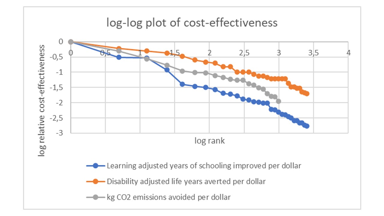
We can take the logarithm (with base 10) of the ratio of the cost-effectiveness of the n-th most effective intervention to the cost-effectiveness of the most effective intervention (i.e. log(xn/xmax)), and plot this against the logarithm of the rank (i.e. log(n)). If the data points are on a straight line, the data follow a power-law distribution.
The figure shows that the cost-effectiveness distributions of the most effective interventions and policies in education, health and climate change, are close to power-laws, as they are almost on straight lines (note however that the data do not allow to reject the possibility that the cost-effectiveness distributions follow another skewed, long-tailed distribution, such as the lognormal distribution). The (least-squares estimate of the) power parameter p equals 0,6 for the education interventions, 1,02 for the health interventions and 1,8 for the climate policies.
In the figure, we see on the vertical axis that the logarithm of cost-effectiveness relative to the most effective intervention ranges up to -2 (for climate policies) and almost -3 (for health policies). This means that the top intervention is 2 or almost 3 orders of magnitude (i.e. a factor 100 and almost 1000) more cost-effective than the least effective intervention. The majority of interventions is more than an order of magnitude less cost-effective than the top intervention.
Why the skewness of cost-effectiveness is important
If the cost-effectiveness distribution of interventions is very skewed, there are two important implications.
First, the information about which interventions are top effective, is very valuable. An effective altruist donor who wants to do the most good by donating to charities, should be willing to pay a lot in order to learn what are the top charities and top interventions. For example, suppose there are 10 interventions, and one of them is 100 times more effective than the other 9. The top intervention does 100 units of good per dollar, whereas the others cause 1 unit of good per dollar. Suppose you have 10 dollars to spend. You can give 1 dollar to each of the 10 interventions, which means you cause 100x1+1x9=109 units of good. Similarly, picking an intervention at random and giving the 10 dollars to that intervention causes 109 units of good in expectation. Without information about effectiveness, you cannot cause more good than 109 units in expectation. But suppose you can pay some money in return for the information which intervention is the best. Paying 8 dollars for this information is worthwhile: the remaining 2 dollar can be spend on the top intervention, causing 2x100=200 units of good, almost twice as much as what you can do without information. You can even pay up to 8,9 dollars for this information, almost 9 times more than what is left to spend on the top intervention. This shows how valuable the information is.
With a power-law distribution, the lower the parameter p, the higher the value of information of cost-effectiveness is and the more important it is to look for more effective interventions. For example, if p=2, and the currently known most effective intervention has cost-effectiveness x, the probability of finding an intervention that is 10 times more effective than x is 1% of the probability of finding an intervention that is barely more cost-effective than x, because P(X>10.x)=C/(10.x)2=P(X>x)/100. But if p=1, the probability of finding an intervention that is 10 times more effective than x is 10% of the probability of finding an intervention that is barely more cost-effective than x. (Sidenote: the expected value of the cost-effectiveness x, given that the new discovered intervention is more effective than the most effective known intervention, is E(x|X>xmax)=C.xmax-p+1.p/(p-1). This expected value approaches infinity when p goes to 1. In reality, there is no infinitely effective intervention, which means the power-law distribution is truncated at the highest value.)
The second important implication, is that if the distribution is very skewed and there may be unknown interventions that are more effective than the interventions you already know, it is worthwhile to look for those unknown interventions and estimate their effectiveness, because it is likely that you find a new intervention that is vastly more effective than the most effective of the known interventions. For example, suppose there are 100 possible interventions, 90 of them cause 1 unit of good per dollar, 9 cause 10 units of good and 1 causes 100 units of good. If you only know about one intervention, that intervention most likely causes 1 unit of good. If you look further, after discovering 6 new interventions, you have probability higher than 50% that one of them causes 10 units of good. Looking further, after discovering 50 interventions, you have probability 50% that one of them is the big winner causing 100 units of good. The more skewed the cost-effectiveness distribution, the more important it is to look further for a more cost-effective intervention. In the explore-exploit tradeoff, a skewed distribution means that one should explore more to look for even better interventions, instead of exploiting the currently known best intervention.
Two notions of scale invariance
There is no well-understood mechanism that explains why many cost-effectiveness distributions are close to a power law. Perhaps it is related to a second type of scale invariance that we see with many power law distributions.
The first scale invariance, mentioned above, relates to rescaling the variable X. Consider the range of interventions with cost-effectiveness between 1 unit and 10 units of good per dollar. Now 10 times more money becomes available, such that with those same interventions, 10 times more good can be done. If the new distribution of how much good can be done with 10 dollar is the same as the old distribution of how much good can be done with 1 dollar for interventions that had a 10 times higher cost-effectiveness (i.e. between 10 and 100 units of good per dollar), then the cost-effectiveness distribution is scale invariant.
But there is a second scale invariance, that relates to hierarchical classification schemes. In a hierarchical classification scheme, a set of elements is subdivided in subsets, which are again subdivided in subsubsets, and so forth. This results in a vertical hierarchy of subdivisions, with the complete set as one group at the top and all the separate elements as different subgroups at the bottom. Each level of subdivisions consists of subgroups. Suppose each of the subgroups at the same level has a property (that is determined by similar properties of their subsubgroups at a lower level). Then we can rank the subgroups, from the highest to the lowest value of that property, and look at the distribution of the property. If the distributions are of the same type for all levels in the hierarchy, there is a scale invariance.
As a concrete example, consider the ways to subdivide the world population in subpopulations. One such division is according to countries, and the population size is a property of a country. So we can consider the distribution of country population sizes. This distribution is close to a power law (with a few outliers, such as India), having estimated power parameter p = 0,9. Now we can consider a country and subdivide it in cities (as if that country is the world and the cities are countries), and look at the distribution of population sizes of the cities in that country. For many countries and many years, the sizes of (the largest) cities also closely follow power law distributions (e.g. for US cities, p=1,02). The power law can also appear on other levels, such as city streets or states (the 35 most populated states in the US roughly follow a power law with p=1,5). Hence, we have a hierarchy of power law distributions. This is a fractal pattern with self-similarity: the distribution at the lower scale of cities is similar to the distribution at the higher scale of countries (and perhaps other scales, such as city streets).
A second example is biological taxonomy. We can divide the set of all living beings in subsets of kingdoms (e.g. animals), which can be further subdivided in phylums (e.g. chordates), which can be subdivided in classes (e.g. mammals), which can be subdivided in orders (e.g. primates), which can be subdivided in families (e.g. great apes), which can be subdivided in species (e.g. humans), which can be subdivided in subspecies (e.g. homo sapiens sapiens), which can finally be subdivided in individuals (e.g. you). At a taxonomic rank (a level in this hierarchy), such as the rank of species, we can observe a power law distribution of abundance (number of individuals belonging to the taxon). For example, the species abundance distribution shows the number of individuals per species. This is a skewed distribution, close to a power law with average parameter p=1,1. A small minority of species are much more abundant than the vast majority of species.
A third example brings us closer to the cost-effectiveness distribution of health interventions. The Global Burden of Disease measures the shares of healthy life years lost (i.e. DALYs) by several diseases. At the highest level, the set of diseases can be divided in major groups such as non-communicable diseases, injuries, nutritional diseases and infectious diseases. At a second level, the group of non-communicable diseases can be subdivided in e.g. cancers (neoplasms), cardiovascular diseases, chronic respiratory diseases, metabolic diseases (diabetes), mental disorders and other non-communicable diseases. Next, cancers can be subdivided into e.g. skin cancer, lung cancer, breast cancers and many others. Skin cancers can be subdivided into melanoma and squamous-cell carcinoma. For many diseases, at many levels, we see DALY distributions close to power laws. For example, at the second level, the distribution of non-communicable diseases has an estimated parameter p=1,2. A level lower, the cancers also have an estimated parameter p=1,2 (whereas e.g. the cardiovascular diseases have p=0,5).
With the above examples, we can hypothesize that power law distributions are common in hierarchical classification schemes. But like diseases, interventions can also be classified in such hierarchical classification schemes. We can subdivide the set of altruistic interventions in e.g. longtermist versus neartermist interventions. Neartermist interventions can be subdivided according to biological taxonomic groups, such as human welfare interventions versus animal welfare interventions. Human welfare interventions can be subdivided according to objective such as health. Human health interventions can be further subdivided according to geography (e.g. country), disease (e.g. skin cancer) or treatment (e.g. prevention campaigns). In the end, we can investigate e.g. the cost-effectiveness of a skin cancer prevention campaign in the US.
Whether hierarchical classification schemes are more likely to exhibit power laws, is an open question for future research. But perhaps it offers (a part of) an explanation why cost-effectiveness distributions are skewed like power-law distributions. (Sidenote: cost-effectiveness distributions can also resemble skewed lognormal distributions. The multiplicative central limit theorem says that the limiting distribution for the product of many independent positive random variables with finite variances, is lognormal. Hence, if the cost-effectiveness is determined by a product of a lot of random factors, we may see a lognormal distribution. Many skewed distributions, such as household income or city sizes, appear to be lognormal in the bulk and power-law in the tail.)
Hierarchical classification schemes, arbitrariness and effectiveness
Hierarchical classification schemes may not only be associated with power-law distributions, but they are also a cause for concern for effective altruists. As argued elsewhere, such classification schemes may generate a moral illusion or cognitive bias of arbitrary group selection, which influences our cause prioritization and makes us less effective.
Nationalists prioritize helping people who are born in their own country. But why their own country and not their own city or their own planet? The choice for the country, i.e. a specific level in the hierarchy, is arbitrary. Similarly, speciesists prioritize helping individuals who belong to their own species. But why their own species and not their own race or their own phylum? Picking the level of species instead of other levels in the biological hierarchy, is arbitrary. Similarly, many people want to support a charity that targets a certain type of diseases, such as cancers. But why prioritizing cancers and not e.g. skin cancers or non-communicable diseases?
Arbitrary group selection bias means preferring or prioritizing an arbitrary group (e.g. the group of fellow countrymen, the group of humans or the group of cancer patients) at an arbitrary level in a hierarchical classification. Sticking to one’s own preferred country, species or disease, is not only arbitrary, but it prevents us from taking opportunities to do more good. One can often do more good by helping individuals who live in other countries, who belong to other species or who have other diseases than cancer. Nationalist and speciesist inclinations make us less effective, and they are a cause of discrimination. The same goes for an inclination to prioritize a certain disease such as cancer. Impartiality or cause-neutrality means that in order to be more effective, one should only look at the top level in the hierarchical classification, i.e. consider the whole world (instead of a specific country), all beings (instead of members from a specific species), and all diseases (instead of a specific type of diseases such as cancers). Especially when we see power-law distributions in cost-effectiveness related to hierarchical classification schemes, an arbitrary group selection bias is a serious cause of a loss of effectiveness.
This is the third in a sequence of posts taken from my recent report: Why Did Environmentalism Become Partisan?
Summary
Rising partisanship did not make environmentalism more popular or politically effective. Instead, it saw flat or falling overall public opinion, fewer major legislative achievements, and fluctuating executive actions.
Public Opinion...
This post presents the executive summary from Giving What We Can’s impact evaluation for 2025. At the end of this post we share links to more information, including the full report and...

Here is one speculation of what could explain the prevalence of heavy-tailed distributions in what you call 'hierarchical classification schemes':
Suppose that the causal mechanism generating the relevant classes has the property that new members are more likely to be added to a class the more members it already has (e.g. if people were more likely to move to a city the higher its population). Under some such conditions it's then a mathematical consequence that the size distribution (i.e. number of members across classes) will converge to a power law.
This has been popularized as "preferential attachment" by the 'network science' people around Barabasi since the end of the 1990s to explain various observations on the Internet and other networks (though the related academic cottage industry has recently received some good criticism). But the maths and potential real-world cases are much older; indeed, the perhaps first major case for which this explanation was proposed was one of your examples - biological taxa -, by Yule in the 1920s.
For a survey of other generating mechanisms of power laws, see Newman (2005) and this blog post by Terence Tao.