Writing my summary of Evidence, Decision, and Causality, I got interested in how EDT might be able to succeed by precommitting, and how different simulation schemes that a predictor might run of the transparent Newcomb’s problem might affect the way EDT and CDT reason about the problem. Precommitments hinge on an aspect of sophisticated choice that I haven’t been able to find information on. Indexical (or anthropic) uncertainty seems to do the trick unambiguously.

Be warned that these things were probably only new to me, so if you know some decision theory you may end up bored, and I wouldn’t want that. (That’s probably also why I didn’t cross-post this to the EA Forum in 2020. I seem to have redecided, but now I’ll be less able to answer questions about my reasoning back in the day.)

Precommitments

In the transparent Newcomb’s problem, CDT and EDT are both said to two-box and fail to become millionaires. Most decision theorists would call me insane (or maybe they’d be more polite about their disapproval) for wanting to one-box in this situation, but maybe I just really like money.

So I wonder whether I need to adopt a UDT-like decision theory to achieve this or whether I have other options, in particular options compatible with following the advice of EDT.

Friends of mine said that EDT would update on the nonoptimality of its approach and choose to precommit. For that to work out, it’ll need (1) a full understanding of the choice situation and (2) a chance to precommit. It’ll need both of these before learning some crucial information, in this case the contents of the boxes. Thereby it would, in effect, implement updateless behavior in individual choice situations.

But I somehow can’t make that happen. I turn it into a sequential choice problem by adding a chance to precommit when the agent knows the choice situation but hasn’t seen the (transparent) boxes. To precommit, the agent puts $1,001 in escrow, which they’ll only get back if they one-box.

I’ll write M and K for the potential money under the boxes ($1,000,000 and $1,000 respectively) and E = $1,001 for the potential amount in escrow. The predictor is known to be perfect, so some cases are impossible. First the myopic case:

Myopic EDT may endorse escrow but there’s nothing here that makes it recommend it over no escrow. The case where the agent gets the million is, by construction, identical to the case where they get the million and get the escrow money back. In practice, precommitments will come with small costs – transaction costs, lost interest, option value, vel sim. – but may still be very much worth it. Yet myopic EDT would then no longer even endorse them.

The sophisticated choice situation is unclear to me. The materials on decision theory that I’ve read didn’t feature a case where the likely payoffs of the final stage of a multi-stage decision problem varied depending on decisions at earlier stages. Usually the preferences changed or nothing changed. EDT normally recommends two-boxing if it encounters the second stage in isolation. If that recommendation were the starting point of the backward induction, it would make the escrow seem highly undesirable.

But at least intuitively it seems unproblematic to me (without a textbook to back me up, I’m afraid I may be overlooking some incoherency) to take the bad news into account that two-boxing confers when it comes to the then-empty box. I just don’t know if this is in the spirit of sophisticated choice or already touches on policy selection. But if this is compatible with how decision theorists typically understand sophisticated choice and EDT to operate, then EDT recommends escrow. The table above is the result of eliminating “escrow, two-box” because two-boxing at the final stage would violate the agent’s preferences, and eliminating “No escrow, one-box” for the same reason and the reason that the actual preferences would make the case inconsistent. What remains is for the agent to choose “escrow, one-box.” Yay! I just hope this way of reasoning is consistent.

Resolute choice solves the issue, but then resolute choice doesn’t require any separate precommitment stage to begin with.

Updatelessness

There is also the consideration that such thorough reasoners as these idealized agents will consider that they have some degree of indexical (or anthropic^[1]) uncertainty. The predictor may determine the agent’s bet conditional on the prediction by running a simulation of them, and the agent may currently be inside that simulation. This consideration would make both EDT and CDT updateless and thereby rich.

For concision I’ll write “one-boxer” for “an agent that has been found to de facto follow the one-boxer policy.” Calling the agent a one-boxer makes it sound like this is an indelible property of the agent rather than an observation. This would be problematic in the standard Newcomb’s problem since such an inherent property is likely to be known to the agent themselves, and then the Tickle Defense would apply to the resulting problem. Here I intend “one-boxer” etc. as mere shorthands without all these implications.

In the transparent Newcomb’s problem, the agents can update on the payoffs in both boxes, so there are four instead of two policies (see the table below):

1. One-boxer: Take one box (the formally opaque one) no matter what.
2. Two-boxer: Take both boxes no matter what.
3. Conformist: One-box if there is a million in the box (M, K); otherwise two-box.
4. Rebel: One-box if the box is empty (0, K); otherwise two-box.

Some Observations

1. It’s unclear what box configuration Omega should choose for conformists or rebels, so a default (M, K or 0, K) needs to be chosen for those cases. 0, K somehow strikes me as the more natural default, but see also point 5 below where I suggest a new configuration 0, 0.
2. There may be different simulation regimes (see the table below):
   1. Simulating both box configurations multiple times (“n sim.”) to capture whether agents follow different policies with some probability. This would need to be real randomness, not some pseudo-randomness that can be simulated. The predictor would then need a separate policy for how to respond to, say, agents that one-box only most of the time. I’ll omit this case here.
   2. Simulating both box configurations once (“2 sim.”).
   3. Simulating one box configuration, and only simulating the other one if the agent makes a decision that is inconsistent (or consistent, but that seems almost equivalent and intuitively odd) with seeing that box configuration (“1.5 sim.”).
   4. Simulating only one box configuration (“1 sim.”) and accepting that you can’t distinguish the conformists and rebels from one of the other strategies.
3. In cases 1.5 sim. and 1 sim. it is important which scenario is simulated first. The resulting differences are in the table below. A bold choice in the 1.5 sim. table means that the simulation completed after a single run. Regular type means that it took two runs.
4. Encoding perfect predictions in the two configurations of boxed money is no longer possible as there are only two such configurations in the original problem. A rebel bot that always follows the rebel strategy could thwart any such prediction. But you could introduce a 0, 0 payoff combination as default (in the above sense) to discourage some strategies that update on the boxed money:
   1. The 0, 0 payoff could await both conformist and rebel. A conformist bot would then see 0, 0 even though they would’ve one-boxed if the payoffs had been M, K.
   2. The predictor could also choose to only use the default for rebels since that is the one policy that would otherwise lead to paradox. The predictor could then randomize what to give to the conformist.
   3. Finally, the predictor could use the (perhaps cheaper) 1.5 sim. regime to determine the payoffs in option b. It won’t be able to tell the conformist from the one-boxer or the two-boxer, but it will recognize the rebel.
5. If you know which strategy you’ll follow, say, because you’ve precommited to it, and you encounter an inconsistent situation, you still can’t exploit your knowledge because, less interestingly, you’ll have precommitted and because, more interestingly, you’d need to behave in two different ways depending on whether you’re in the simulation or outside, but you can’t because you don’t which is which: If you’ve secretly and nonbindingly committed to two-boxing, and you see M, K, it may be because you’re in a simulation and should one-box or because you’ve one-boxed in the simulation should now really two-box. I’ll mention another reservation later.

Simulation Regimes

2 Sim.

In one column the M, K configuration is tested first and then the 0, K configuration. In the other column the order is reversed. It makes no difference in this case – the resulting configurations are all the same.

1.5 Sim. (Consistent)

In each column, the second configuration is now bracketed because it is only tested if the agent behaved inconsistently in the first configuration. If they behaved consistently right away, the simulation is complete and the resulting configuration is bolded.

1 Sim.

With a single simulation, the conformist and the one-boxer, and the rebel and the two-boxer behave the same if only the M, K configuration is tested. Otherwise, if only the 0, K configuration is tested, the one-boxer and the rebel, and the two-boxer and the conformist behave the same.

Reasoning Under Indexical Uncertainty

There are two things that I’m uncertain about:

1. The materials on decision theory that I’ve read didn’t feature a case where the payoffs of the final stage of a multi-stage decision problem varied depending on decisions at earlier stages. So here I hope that a sophisticated agent (as opposed to a myopic or resolute one) will foresee in earlier stages that they’ll, at the final stage, prefer to be in one rather than another decision situation. I don’t know whether this is actually in accordance with the definitions of the terms.
2. I’m also not clear on whether decision theoretic agents can realize that all their copies will make identical decisions in identical situations (regardless of the stage).

But if this is all the case and maybe also if only the first assumption is true, it seems to me that the argument that EDT and CDT one-box if they realize their indexical uncertainty goes through for this transparent Newcomb’s problem:

First, even if the probability an agent assigns to being in a simulation were small, the opportunity to causally increase the final payoff by a factor of 1,000 by one-boxing would overwhelm even such rather small probabilities.

Second, the probabilities are actually greater than 50%, so substantial. The self-sampling assumption (SSA) and the self-indication assumption (SIA) agree in the case of 2 Sim. and assign probability ⅔ to being in a simulation. (See, e.g., Anthropic Decision Theory.) In 1.5 Sim. they diverge: I’ll assume that the agents have a flat prior over whether the predictor starts by simulating 0, K or M, K. This uncertainty is indicated by the configurations in bold vs. in square brackets in the graphic below.

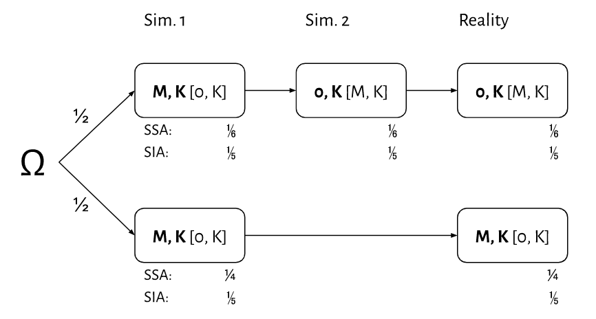
At each stage you see the content of the boxes, so if it is M, K (without loss of generality), you’re either (1) in the bold sim. 1 case at the top, (2) the bracketed sim. 2 case at the top, (3) the bracketed reality case at the top, (4) the bold sim. 1 case at the bottom, or (5) the bold reality case at the bottom. (Hence the SIA probabilities of  each.)

A few reservations and simplifications:

1. I ignore “rebel” agents in this example as they could know for certain that they’re not in one of Omega’s simulations if they see 0, 0. That would make things more complicated.
2. What would also make things complicated are agents who have a strong inclination to one- or two-box and are aware of it. For example, an agent with a strong inclination to one-box may be surprised to see 0, K and so conclude that it’s even more likely to be in a simulation than its SSA or SIA prior implies. Conversely, having a strong inclination and seeing a configuration that is consistent with it may boost once confidence that one is not in a simulation. If the inclination is to one-box (with loss of generality), that might make two-boxing more attractive again, thereby undermining the very inclination to one-box. This seems complicated. Agents with no particular initial inclination (or that are not aware of it) seem to be a simpler case.^[2] Adding up the fractions yields an SSA probability of  and an SIA probability of  in favor of being in a simulation.

I’ve wondered whether there is a way to tweak the payoffs of two-boxing such that an agent that doesn’t take into account that they can’t act differently depending on which stage they’re at can be tricked into making a nonoptimal choice, but I haven’t found one yet.

My main caveat, as mentioned above, is that I’m uncertain over whether CDT and EDT realize that they’ll make the same recommendation in the same situation regardless of the stage. But if that’s the case (and maybe also if not), it seems to me that this argument checks out and indexical (or anthropic) uncertainty really lets CDT and EDT one-box in the transparent Newcomb’s problem.

1. ^{^}

   Is there a difference? I use “indexical” because it seems more self-explanatory to me.

2. ^{^}

   This might be related to the metatickle defence. I haven’t read the paper, though.