Cross-posted from my blog: xabier.me. First post of a series on ARC's AlgZoo networks.
1. The Leeuwenhoek Context.
I’ve decided to name the project after Leeuwenhoek, a pioneer of microscopy who identified thousands of tiny creatures—“animalcules”—in a single drop of water. Our “animalcules” are neural networks.
ARC (Alignment Research Center, an AI safety lab) published a series of tiny networks ranging from 8 to 1,408 parameters—which are “tiny” compared to the models we have today. These networks had been trained to perform very basic tasks, such as finding the second-largest number or the median. They think that if we can’t understand networks as small as these, how are we going to understand ones with billions of parameters? It makes sense if you stop to think about it, and they raise a very interesting challenge.
When I was reviewing their progress and contributions, I noticed that many people were focusing on a family of AlgZoo models, specifically 2nd_argmax (ARC already has a pretty good grasp of its 32-parameter network, which isn’t this one), and that, from what I’ve been able to find (November 2026), argmedian hadn’t been publicly explained yet—so here we are.
2. What It Does
The network receives three numbers, (x1, x2, x3), and says which of the three is the median. It’s a recurrent neural network, meaning it reads the three numbers one at a time and stores the necessary information in four neurons. It has a total of 32 parameters and gets it right 98.46% of the time. We’re going to answer two questions: how does it do this with just four neurons, and why does it fail 1.54% of the time? We’re not focusing on the 98% success rate—we want to see where it fails and why.
3. Where It Fails
The first thing I noticed was that the network has no biases; that is, if we multiply all the numbers by the same value, the neurons and the output scores are multiplied by that number, but the answer does not change. Two sets of proportional numbers, such as (1, 2, 3) and (2, 4, 6), yield the same answer.
This shows us that the network really only cares about the direction of the vector, not its magnitude. Now, since the inputs are independent standard Gaussians, we know that all directions are equally likely; this, in turn, means that the network’s accuracy is a percentage of the surface area of a sphere. So we visualized it by assigning colors to each point and marking the errors in white.
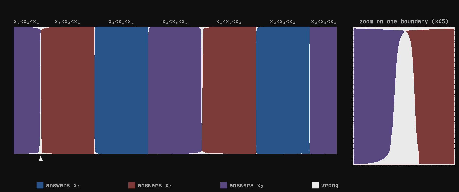 Every input direction on one map, each pixel equally likely. Colour is the answer, white is an error. Errors hug the six boundaries where two numbers tie (zoom on the right).
Thanks to this, we observed that the errors were very thin lines that coincided almost exactly with the boundaries where two numbers were tied. In other words, the network seems to make mistakes only when two numbers are nearly identical.
Then we saw that 77% of the incorrect answers were x1; for some reason, the network gravitated toward the x1 position.
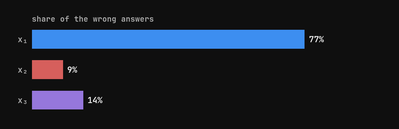 Where the wrong answers go, computed exactly from the weights: 77% of them are x1.
We then observed how the neurons reacted by seeing which ones fired at each step. Upon observation, we found that the four neurons turned out to be two mirror-image pairs. What this means is that one pair fires when the number has increased compared to the previous step, and the other fires when it decreases. Since there are 3 inputs, the network evaluates 3 increases or decreases (in the first step, it compares x1 with 0, so the last two are the ones that matter); this gives us a very clear idea of the network’s strategy. When the number goes up at step 2 and again at step 3—or vice versa (down and down)—we know that the median is always x2. But when the changes are alternating—that is, it goes up first and then down, or vice versa—x2 becomes an extreme, and the network compares x1 with x3.
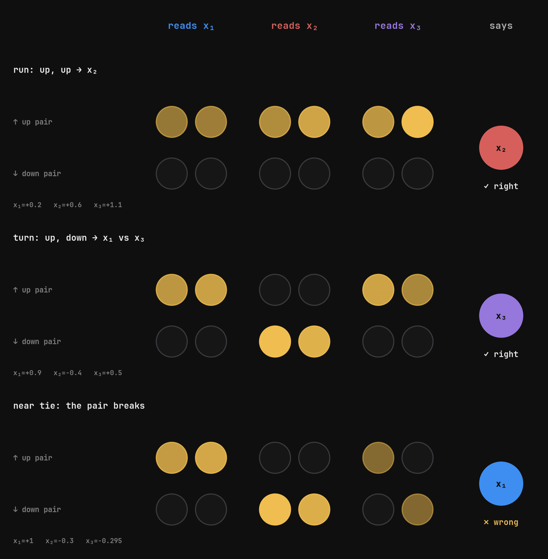 The four neurons at each step, as lamps. A run keeps the up pair lit; a turn switches pairs; near a tie one neuron of each pair stays on and the answer falls back to x1.
Here we run into a problem: the network must remember x2 if it wants to evaluate whether x3 is higher than x2, but it only has 4 neurons, and at each step, one pair is activated. Each pair has two channels. If, instead of looking at one neuron and then another, we look at their sum and their difference, we realize that the sum is the comparison channel. From this, we determine its sign, which tells us whether the value went up or down. The difference is the memory channel—much smaller than the comparison channel—and the network uses it to reconstruct the previous number needed for the next comparison.
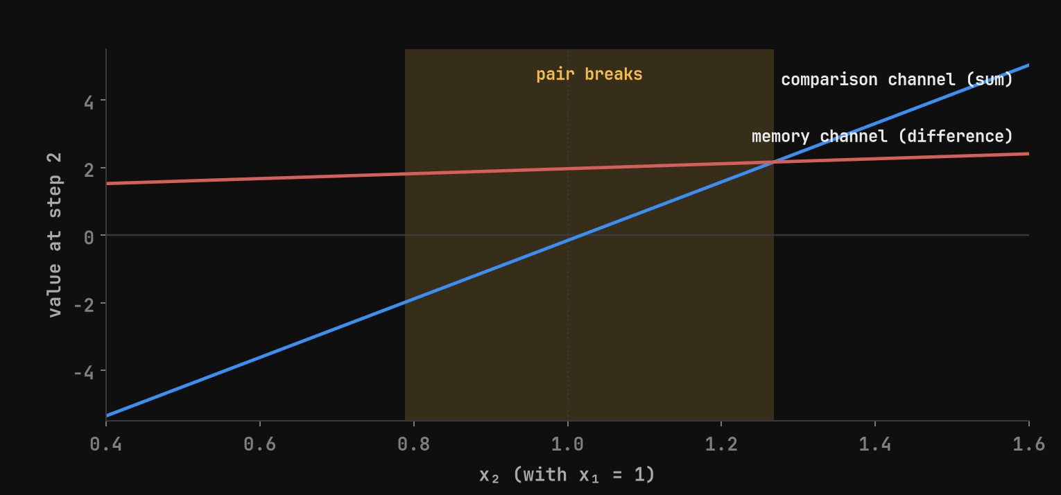 Step 2 with x1 = 1. The comparison channel crosses zero at the tie; while it is smaller than the memory channel, the pair breaks (shaded). It only becomes a wrong answer in a much thinner band.
Knowing this, we return to the problem of ties: when two numbers are nearly equal, the comparison (the first channel) remains nearly zero, and since it is smaller than the memory channel, the neuron pair breaks apart, leaving one neuron from each pair active—as if the network were hesitating—or all of them turn off. When there is a tie, the network tends to choose the first position, x1; that is why the network tends to err more toward x1.
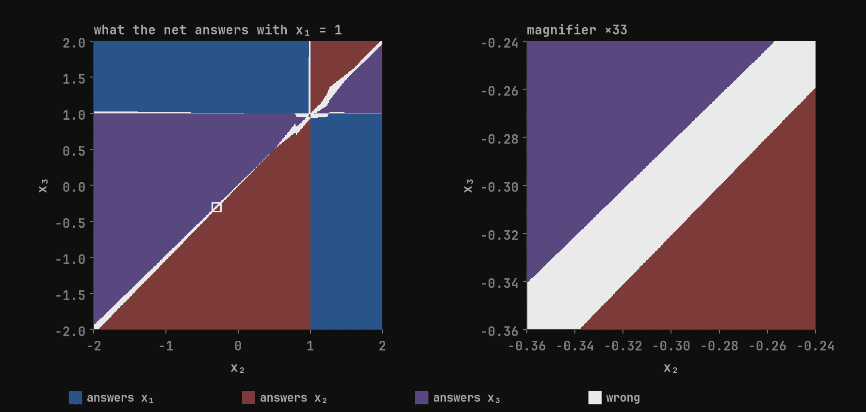 Every (x2, x3) with x1 = 1. The light line along the diagonal is the tie band; the magnifier on the right shows it is a band of constant relative width, not noise.
4. Closing the loop
I only consider an explanation valid if it can be used to create a twin that behaves exactly like the network. The first twin was the first strategy we discussed. It matched the network on 98.46% of the inputs—which is exactly its accuracy rate—which makes sense since that rule is the perfect median, so it only matches exactly where the network gets it right.
To account for the errors, we gradually added the zones where the network failed, each derived from its weights: the tie zone, the shifted boundaries, and where everything shut down. The match rate was 98.82% and gradually reached 99.83% with 22 zones.
We pushed a little further, and with 150 zones we reached 100%, matching the network’s results for 4,000,000 inputs; but to be honest, this was just copying calculations and didn’t add any value, so we focused on the 22 zones.
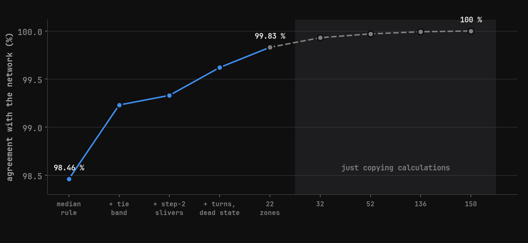 Each twin against the network. The first four steps are mechanisms; after 22 zones it is just copying calculations until the match is exact.
Next, we moved on to the ARC metric, which checks whether an explanation estimates the accuracy better than testing the network on random inputs. We determined the network’s exact accuracy without testing it even once; within each combination of active neurons, the network only adds and multiplies, so what we did was go through the 70 possible combinations and sum the area of each segment of the sphere—this gave us 98.455038%.
The result was obtained by brute force, and we did it this way to get the exact figure against which to measure ourselves.
We then estimated the accuracy by focusing solely on the error we had explained, adding up the areas of those zones. The first estimate was off by 0.52 points from the exact value, and the last one by 0.15. If we calculate it, we find that we would need roughly 6,300 random samples to achieve the same precision by testing it at random.
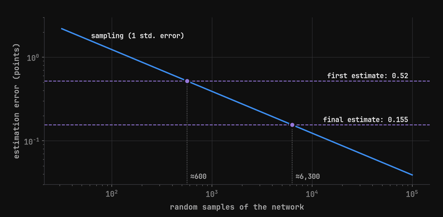 How many random samples it would take to match each estimate. Our estimates come from the weights alone, without running the network.
The previous twin relied on the network’s weights, so we had to build a network based solely on the explanation. To do this, we defined the conditions: that the comparison be exact, that the memory store only what was necessary to reconstruct the previous number, and that the output apply the median rule. Upon solving it, we realized that all the weights had been fixed except for the memory size and the amount forgotten. And this is when we encountered a surprise: by reading the memory size and the amount forgotten from the trained network, the formulas predicted the rest of its weights. One of them was -1.346 (predicted) versus -1.350 (trained). The network built this way achieved 98.52% accuracy, while the original achieved 98.455%.
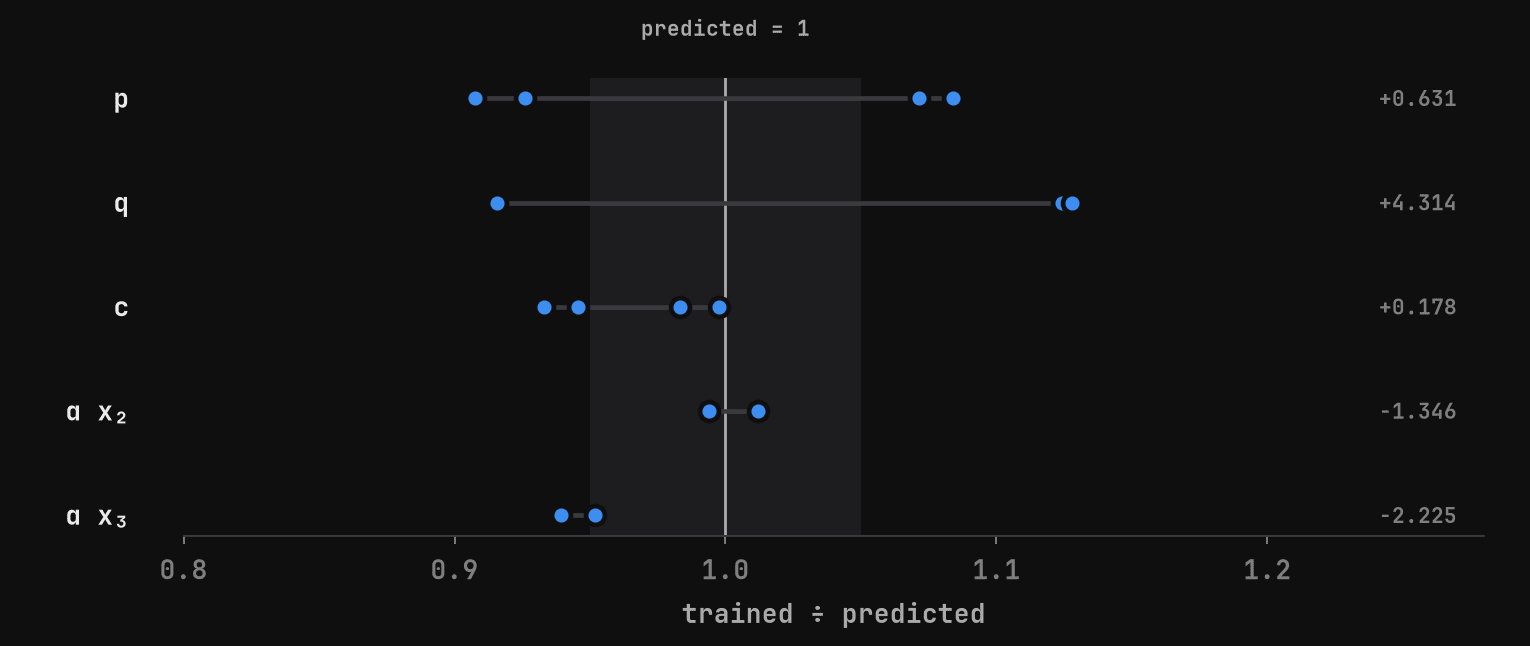 Constants the design predicts from the memory size and how much it forgets, against the trained network (one dot per place each appears). The spread in p and q comes from the trained net forgetting slightly differently within and across halves.
Based on what we've seen so far, I'm surprised at how complex a network with so few parameters can be, and I can't even imagine delving into those with billions of them—especially since, with just 32, the network is capable of separating comparison from memory, and the explanation is able to predict its weights. The 150 zones required to reach 100% aren’t really something from which you can draw any conclusions or gain insight; they’re mere calculations that aren’t worth pausing to understand.
With all this, we know that the error of the built network follows an exact law—with a smaller memory, the network would be correct 99.999% of the time—and why the training ended up with a much larger memory is still unclear.
In the next post, we’ll look at that error law, a recap of the entire process, and more surprising findings.
Claude Code wrote the code and a summary of the results I started with; the text is mine and was translated using DeepL.
Code: https://github.com/Xabilimon1/leeuwenhoek