It is so helpful to have this overview assesment in concentrated form.
In public debates about the pros & cons of economic growth in rich countries there is often the idea "Growth in rich countries is unimportant/bad -- but, yes, for poor countries it is important to still grow".
The kind of work you portray about spillovers puts the viability of the idea "growth in poor countries without growth in rich countries" into question and helpfully puts numbers on how strongly growth in rich countries is linked to growth in poor countries.
I'm curious if anyone has seen research or thought about the inverse, Poor to Rich country spillover effects. While the findings in this post are promising, I worry that they may further incentivize under-investment in international development, as I am similarly worried about efforts to increase high-skill immigration to developed countries, which I fear benefits rich countries at the expense of poorer ones. These are just intuitions though, so I'm not sure if these concerns are unfounded.
How do changes in rich world economic conditions affect poor countries?
AI Use Note: Main body text entirely human written. Claude (Opus 4.8) helped develop models of animal life histories in the appendix.
Cross-posted from Good Structures.
Executive Summary
* Animal advocates sometimes make claims like “there are X of this animal...
“How long have you been v*g*n?”
This is one of the most common icebreakers at animal protection events. It’s a baseline assumption, and it mostly holds true: if you’re out advocating for animals not to be tortured or abused, realistically these days you are v**n, or close. And it makes for good conversation. It seems fairly safe to assume when you meet strangers.
But this assumption is hurting the movement in a way which we don’t always notice: someone new comes into the sp...
Summary
Back in November 2023 I posted here to launch Spiro and raise our first $198k. Two and a half years later this is an update and a fundraiser for the next step.
The short version: we've now reached over-5,900 people with TB preventive medicine, including over 3,000 children under five years old. Our early results have held up well an...
This essay was submitted to Open Philanthropy's Cause Exploration Prizes contest and posted to the Forum with the author's permission.
If you're seeing this in summer 2022, we'll be posting many submissions in a short period. If you want to stop seeing them so often, apply a filter for the appropriate tag!
I. Summary
Investigating rich to poor country income spillovers, we find consistently significant and positive elasticity estimates. We look at elasticities stemming from macroeconomic policy changes and new technologies increasing productivity, as well as between aggregate rich world and LMIC GDP.
Specifically, we find…
Rich world income growth produces rich-poor income elasticities ranging from 0.5 to 1, on average, according to the academic literature addressing this question.
The short-run elasticity between short-term US interest rates and LMIC GDP growth is at least -0.5 percentage points, and likely more negative in the short-term.
There is a need for further research on the potential second-order effects of lower interest rates, especially in the medium to long term and when modeling the impact of full employment advocacy in the rich world.[1][2]
New technologies have an income elasticity of 1 if the technology is deployed in both rich and poor countries, but an income elasticity of 0 (no increase in poor country income) if the technology only gets deployed in rich countries.
This last finding leads us to conclude that transferable sources of rich world productivity growth (e.g. general purpose technologies) will produce significantly greater LMIC spillovers than allocational productivity gains that can’t easily be translated globally (e.g. YIMBY successes).[3]Allocational gains in the US are welcomed, but if maximizing LMIC income spillovers is the goal, it is somewhat intuitive that new productivity enhancing technologies that can be deployed abroad, even with more uncertain lags, are more effective.
II. Rich world → LMIC growth spillovers
We start by reviewing the literature that directly estimates rich world GDP growth spillovers to low-and middle-income country GDP. We use GDP as a proxy for income because the available research and data availability focuses on this measure.[4] We find an average rich-poor income elasticity ranging from around 0.5 to 1 on average. This estimate is primarily based on a literature review of academic and policy papers produced by well-regarded research institutions.
Different research organizations have published fairly transparent reports estimating rich world to low-and middle-income country (LMIC) GDP spillovers. Note that these papers are predominantly produced by the World Bank. If their methodology is systemically unsound, it would pose a key uncertainty for these estimates.
The research (summarized in Appendix A) make use of several types of vector autoregression (VAR) methods that relate historic macro variables (e.g. interest rates, growth rate, global oil price, etc.) across countries or regions to estimate the likely response of a shock in one country to another region of interest. For example, a researcher may be interested in the impact a 1% boost to US GDP may have on a sample of Asian economies' growth. Using VAR the modelers "shock" the US's GDP by 1% then simulate the response of their sample Asian economies GDP in the future. It's important to note that these models are not necessarily holding other advanced economies growth constant, so these simulated impacts may include the second-order spillovers from other advanced economies in response to a US growth shock. Despite their more correlational focus, VAR models are widely used for the impulse response applications presented in this memo.
Estimates vary, but elasticities are consistently positive across the advanced economies considered (Europe, advanced economy samples, and the US).[5]Elasticity estimates for emerging economies range from 0.3–1 when the shock originates in Europe, 0.8–2.2 when originating in a collection of advanced economies (typically the G7), and 0.4–1.6 when originating in the US. The results appear intuitively consistent, with Europe and the US producing similarly sized spillovers of 0.8 on average, while slightly higher, the grouped advanced economy average elasticity in this sample of papers was 1.3. The difference amongst these estimates stem from the use of different spillover recipient samples, different data year coverage, and slight differences in their models.
It’s important to note that these papers tend to exclude the lowest income countries, especially those in Sub Saharan Africa (SSA), from their modeling. This omission likely stems from a combination of SSA's relatively low share of world GDP, a lack of reliable data, and a general disinterest on the part of developed country researchers. Whatever the reason, this omission is important because extreme poverty is currently concentrated, and likely to continue concentrating, in SSA as Asian countries continue successful poverty reduction efforts.[6][7] To provide an approximation of relative economic connection, and thus likely relative size of GDP spillovers, we have summarized exports and foreign direct investment between the world's poorest regions and the US, Europe, and China in Table 1.[8][9]
Table 1: Trade and FDI linkages with highly impoverished regions, 2019
Region
Population in poverty
(millions of people, $3.20/day)
USA
EU27
China
Share of exports (%)
Share of inward FDI
(%)
Share of exports (%)
Share of inward FDI
(%)
Share of exports (%)
Share of inward FDI
(%)
Sub-Saharan Africa
7,162
5
12
23
36
16
3
India
689
17
17
17
40
5
0
Bangladesh
85
15
21
47
25
2
5
Pakistan
74
17
5
35
54
9
8
Indonesia
54
11
13
9
20
17
3
China
24
17
3
17
8
-
-
Notes: Trade linkage is represented by the share of the poor country’s exports that flowed to each major economy. Investment is represented by the share of total inward FDI stock in the poor country contributed by each major economy.
Sources: World Bank, IMF, World Integrated Trade Solution, Trading Economics, Macro Trends, U.S. Trade Representative
To illustrate, the EU recently imported 23% of SSA’s exports and provided 36% of their foreign direct investment stock. The US imported only 5% of SSA’s exports and contributed 12% of foreign direct investment by 2019. Because of this substantial difference in two impactful economic linkage metrics, the EU's growth spillover to SSA may be higher than the spillover resulting from a similar growth shock in the US.
Compared to the US, the EU appears to be more economically connected to the world’s poorest regions in terms of foreign direct investment in particular, and equally or more connected in terms of trade. China still lags the US and EU in economic connectedness to the most impoverished countries highlighted in this memo, with the one notable exception being China’s trade relations with SSA. We only reviewed the literature related to rich world growth shocks for this project, but as China's shares of world GDP and trade with Africa continue increasing, China's growth spillovers will likely increase in importance as it relates to spillovers in low income areas.[9]
Robust modeling needs to be done to gain more confidence, but these linkages may provide a useful approximation of potential relative spillovers for those areas currently excluded from spillover modeling.
Next, we examine two spillover mechanisms in detail.
III. Specific spillover mechanisms: Macroeconomic policy and Productivity
The two spillover mechanisms of particular interest to OpenPhil, macroeconomic policy and productivity shocks that boost rich world growth, both explain a share of the documented spillovers established in Section II. We conservatively estimate that a 1% increase in US interest rates will result in at least a decline of 0.5% in GDP growth within a year of monetary tightening in LMIC. We also estimate that productivity gains in the rich world produce income elasticities near 1, while productivity gains that don’t diffuse globally produce slightly negative elasticities near 0.
III.A. Macroeconomic policy
Macroeconomic policy in the rich world, especially in the US, has considerable influence on the global economy, beyond any direct impact on American growth. Researchers find a consistently negative relationship between higher US interest rates and LMIC growth rates. We conservatively estimate that a
1% increase in US interest rates will result in at least a decline of 0.5% in GDP growth within a year of monetary tightening in LMIC.[10]We are fairly certain this is a conservative estimation of the rich world interest rate-LMIC income elasticity in the short-term, but are uncertain about the potential long run impacts of easy money globally. The main source of this estimate is a review of the academic literature that relates US interest rate shocks to LMIC GDP.
All of the papers we reviewed that included readily interpretable elasticities focused on rate hikes in the US, opposed to monetary loosening or other central banks’ decision making. These papers focused on the impact of both short and long term rate changes on international output, either through GDP, GDP growth, or industrial production. Cumulated response times for these monetary spillovers ranged from immediate impact to 4 years. It is also important to note that the shock mechanisms in these models were more varied than in the direct GDP spillover research. Some researchers shocked the federal funds rate (short-term rate) directly, while others adjusted different economic levels to obtain a resulting simulation with a desired rise in a 1 year treasury yield, for example. We have presented the elasticity between the output metric and the monetary rate that was eventually raised in Appendix B.
Estimates of the impact on emerging market output of a short-term rate increase in the US of 1% ranged from a decline of 0.2% in the markets less exposed to exchange rate risks, to a fall in industrial production of 4% in more financially open markets. The most severe contraction predicted by a US monetary shock to a long term rate came from an IMF paper where EM GDP was estimated to be 0.7% lower than GDP at the time of the shock, four years after a 1% increase in the 10-year US treasury yield. The one paper that presented a positive elasticity between US monetary tightening and EM output modeled a rate hike that coincided with strong US growth. In that case, the effect of strong US growth outweighed the negative impacts of higher interest rates.
Comparing these elasticities is difficult because of the various rates and output metrics considered across studies. The results we considered also vary sufficiently to make precise elasticity estimates uncertain, with some estimates only suggesting a less than 1% reduction in the output growth rate, while others suggesting a decline greater than 0.5% in the output level. However, the relationship between tighter US monetary policy and EM output is consistently negative in the results we reviewed. All considered, we believe it is reasonable to conservatively estimate that a 1% increase in US interest rates will result in at least a decline of 0.5% in GDP growth within a year of monetary tightening, with median effects likely more severe. Note that this research measures elasticities between US rate increases and LMIC output. The measured effects don’t necessarily all flow through higher US output and demand growth. It is more likely that the bulk of such effects are direct spillovers resulting from the dollar’s pivotal position in international finance. As such, these estimates may be more useful when making grants to advocacy groups focused on full employment and lower rates in the US, opposed to calculations interested solely in rich-poor income elasticities.
It’s clear that US downturns caused, or accompanied by, higher US rates are associated with reduced growth in LMIC.[11]However, there is a chance that low rates contribute to higher inflation and excessive borrowing, both of which can decrease stability and trigger rate hikes in the future.
For example, low interest rates in the US provide liquidity and credit globally that spurs LMIC growth. This increased credit supply can potentially cause inflation and increase debt in LMIC. When inflation in particular picks up, the Fed will likely raise rates some amount. Any rate hike will likely decrease LMIC economic growth as rich world demand, trade, and capital flows decline.
The logic is necessarily circular but we are not confident in the empirical trade off between the immediate impact of lower rates versus the increased probability of instability in the future due to a previous period of low interest rates. We have not done an exhaustive literature review on this topic, but from what we have reviewed, we haven’t seen research estimating this trade off. Attempting to better quantify this potential second-order effect is worth considering. A slightly longer note on these risks can be found in Appendix B.
Productivity shocks are shown to be another key spillover mechanism between rich world economies and LMIC output.
III.B. Productivity
To estimate GDP spillovers, specifically due to technological change, we use a theoretical economic model to estimate rich-poor country income elasticities. We find that short-run elasticities are around -0.1, while long run elasticities (years to decades) are around +1.0. While the aggregate elasticity and interest rate elasticity were primarily based on academic papers, this estimate stems from our model of the world economy described below.
The specific model used is the Standard GTAPmodel.[12]Overall, the Standard GTAP model attempts to create a realistic picture of the entire world economy. Our implementation of the model contains 10 different sectors of the economy, ranging from agriculture to manufacturing to services. As is typical in economic models, output of each commodity is produced using “endowments” or “intermediate inputs”. The endowments are quasi-fixed resources such as capital, labor, land, and natural resources. The “intermediate inputs” are each of the 10 commodities and their level of output, location of production, and which sector they are assigned to is completely flexible. There are two regions: high income countries and low income countries. Income accrues to households in each region based on the amount of labor, capital and other endowments that they supply, and the price or wage that they receive for those endowments.
This analysis estimates the rich-poor country income elasticity by looking at 10 different scenarios, each with a slightly different type of technological change or technological diffusion. First, the scenarios either assume that the technology is deployed only in rich countries (no tech diffusion to poor), or equally in both rich and poor countries (full tech diffusion). Second, the scenarios shock one of 5 slightly different productivity parameters. As previously stated, in the model, output of each commodity is produced using capital, labor, and intermediate inputs. The 5 technological shocks correspond to increasing the productivity of some subset of these inputs, and seeing the resulting impact on rich and poor country income.
Specifically the 5 shock options correspond to increasing the productivity of:
All endowments and intermediate inputs (ie, combining 3 and 4)
When these 5 options are combined with the 2 technological diffusion options, that gives a total of 2 X 5 = 10 scenarios. For more model details please see Appendix C.
We look at a variety of productivity options because it is often hard to predict whether a particular technology will increase the productivity of capital, labor, intermediates, or some subset. For example, consider an improvement in the technology for cutting sheet metal. A new technology might improve the accuracy of a machine that cuts sheet metal, reducing the intermediate inputs needed for a given unit of output (and thus increasing intermediate input productivity). Alternatively, the new technology might allow the machine to cut more quickly, requiring less machines to be used (and thus increasing capital productivity). Or it might allow for the output of one machine to be directly fed into another, without manual handling (and thus increasing labor productivity).
Overall, the impacts of a productivity shock are overwhelmingly domestic, substantial “spillovers” only really occur when other countries also deploy that technology. If a technology never diffuses to the poor world, the technology has small negative impacts on those countries: elasticities are around -0.07 (see the left column of table 2). But in the scenarios with full technology diffusion (rightmost column), elasticities range from 0.9 to 1.3. Given a path of diffusion, there is not much difference in elasticity between the different channels of productivity that can be increased (top vs middle vs bottom rows).
Table 2: Elasticity of Poor Country GDP with respect to Rich Country GDP, under various technology diffusion assumptions and types of productivity increases
Technological diffusion (right vs left column) seems to be the key parameter that determines how much a technology impacts poor country income. In general, it seems like all technologies eventually diffuse to the entire world but this process can take years or decades.[13][14] This likely means that technologies have a “short-run” elasticity of around -0.1 but a long run elasticity of around 1.0, with the exact time period that defines “short” and “long” run varying with the technology, but varying from several years to several decades.
The main potential downside to this model’s accuracy is that it doesn’t include monetary channels or a nuanced modeling of interconnectedness in the global financial system. The model does include a financial sector, but not all of the monetary plumbing connections and idiosyncratic behavior observable in actual markets that are due to human emotion. This may be important because economic downturns in particular are often transmitted through sticky prices and financial and confidence channels.
Bibliography for literature reviews
Ahmed, Shaghil, Ozge Akinci, Albert Queralto (2021). “U.S. Monetary Policy Spillovers to Emerging Markets: Both Shocks and Vulnerabilities Matter,” International Finance Discussion Papers 1321.
Alejandro Vicondoa (2019). “Monetary news in the United States and business cycles in emerging economies,” Journal of International Economics, Vol 117, p. 79-90.
Arezki, Rabah and Liu, Yang (2018). “On the Asymmetry of Global Spillovers: Emerging Markets Versus Advanced Economies,” Policy Research Working Paper 8662, World Bank.
Bilge Erten (2012). “Macroeconomic Transmission of Eurozone Shocks to Emerging Economies,” Centre d'Études Prospectives et d'Informations Internationales.
Franz Ulrich Ruch (2020). "Prospects, Risks, and Vulnerabilities in Emerging and Developing Economies: Lessons from the Past Decade" Policy Research Working Paper 9181, World Bank.
Iacoviello, Matteo and Gaston Navarro (2018). “Foreign Effects of Higher U.S. Interest Rates,” International Finance Discussion Papers 1227. Board of Governors of the Federal Reserve System.
Ozge Akinci and Albert Queralto (2021). “How Does U.S. Monetary Policy Affect Emerging Market Economies?” Liberty Street Economics, Federal Reserve Bank of New York.
Notes: EMDE = Emerging markets and developing economies, EM = Emerging markets, AE = Advanced economies, FM = Frontier markets.
B. Macroeconomic policy
Macroeconomic policy spillover literature review
Source
Year
Area shocked
Spillover recipients
Monetary shock variable
Response metric
Elasticity
Cumulated response time
Short-term rate shocks
Akinci and Queralto (Federal Reserve)
2021
US
EM
Federal funds rate
Real GDP
-0.45
2 years
Ahmed, Akinci, Queralto (Federal Reserve)
2021
US
EM (vulnerable)
Federal funds rate
GDP
-0.4
2 years
Ahmed, Akinci, Queralto (Federal Reserve)
2021
US
EM (non-vulnerable)
Federal funds rate
GDP
-0.2
2 years
Degasperi, Hong, Ricco (University of Warwick)
2021
US
EM (more open)
1-year Treasury
Industrial
production
-4
1 year
Degasperi, Hong, Ricco (University of Warwick)
2021
US
EM (median)
1-year Treasury
Industrial
production
-2.5
1 year
Degasperi, Hong, Ricco (University of Warwick)
2021
US
EM (less open)
1-year Treasury
Industrial
production
-0.5
1 year
Vicondoa (Journal of International Economics)
2018
US
EM
Anticipated federal funds rate hike
GDP
-2
Immediate
Long term rate shocks
Iacoviello and Navarro (Federal Reserve Board)
2018
US
EM
10-year real rate
GDP
-0.7
4 years
Druck, Magud, Mariscal (IMF)
2015
US
Central America and Mexico
10-year real rate
Real GDP growth
-0.4
1 year
Druck, Magud, Mariscal (IMF)
2015
US
MENA
10-year real rate
Real GDP growth
-0.3
1 year
Druck, Magud, Mariscal (IMF)
2015
US
South America
10-year real rate
Real GDP growth
-0.6
1 year
Kose, Lakatos, Ohnsorge, Stocker (World Bank)
2017
US
EMDE
Long term interest rate spike
accompanied by US growth
Industrial
production
1.2
?
Kose, Lakatos, Ohnsorge, Stocker (World Bank)
2017
US
EMDE
Unexpected long term interest rate spike
Industrial
production
-0.2
?
Note on macro policy uncertainty:
The evidence that rate hikes hinder LMIC growth, does not necessarily mean that lower US interest rates are an unmitigated good for LMIC economic growth. Low US interest rates provide increased liquidity for trade and investment, but this lubrication simultaneously increases reliance on global dollar funding in LMIC which can reinforce sizable economic risks.
When LMIC rely on significant foreign capital flows for investment financing and/or trade credits, low interest rates blow strong wind in their economic sails. The issue is that capital flows into LMIC are typically the last in and first out when the weather gets rough. This can result in sudden and destabilizing capital outflows that are associated with a roughly 4% decline in GDP growth in the following year.[15]
These shocks have the potential to negate years of smooth sailing in a short period of time, as seen in the Asian Financial Crisis where years of increased capital inflows quickly reversed as foreign investor confidence evaporated with the breaking of Thailand’s currency peg in 1997. Bad weather for LMIC capital flows can stem from multiple sources, but one of the most relevant is Federal Reserve interest rate changes.
The US dollar’s central, and outsized, role in global finance amplifies the international spillovers from every decision the Fed makes. Roughly 50% of all cross-border loans are made in dollars.[16]When the Fed raises interest rates it mechanically increases the servicing cost of all variable rate instruments. Even fixed rate dollar loans are often rolled over multiple times in floating rate markets, consequently exposing these loans to interest rate hikes too. This exposure is typified by the 1980s debt crises, where predominantly Latin American sovereign borrowers were caught off guard by the increased debt servicing costs following the “Volcker shock”. The interest rate shock was named after the Fed Chair who hiked interest rates to near 20% to subdue a decade of inflation in the US. The preceding debt build up in the 1970s was caused primarily by the savings glut from Middle Eastern-oil-rich countries that was recycled into Latin America. However the financial environment encouraged borrowing with real interest rates close to zero throughout this period.[17]The dollar denominated borrowing was well and good until an external shock (a Fed rate hike), totally out of the control of Latin America, sank many of the region’s countries under the weight of untenable debt servicing costs in what many call the “Lost Decade.” Borrowing in a country’s own currency limits the government to domestic credit markets, but also provides it more monetary policy autonomy. Debt distress is on the rise once again and will likely continue to disproportionately impact LMIC as long as external borrowing remains relatively cheap, at least in the short-term.[18]
US dollar trade poses a similar fragility for LMIC growth. Roughly 50% of all trade is invoiced in US dollars, despite the fact that US trade accounts for only ~10% of the world total.Final transactions are often priced in dollars, but importers and exporters also often finance their businesses using dollar credit. Unexpected increases in US interest rates can sap global dollar liquidity and reduce the available dollars for selling final goods, but also for inputs and intermediate investments needed by LMIC producers.
Researchers show a striking negative relationship between global trade flows and dollar strength, highlighting the dominance of the financial channel in the impact of US rate changes on LMIC trade.[19]
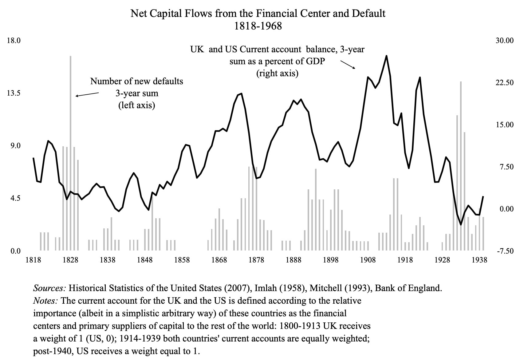
These fragilities have been present in history whenever peripheral countries rely on a “core” country for global credit. Before its rise to its current status, the US’s three largest financial panics in the 1800s were at least partially attributable to changes to financial conditions in the core country of the time, England. This pattern can be seen in Carmen Rienhart and Kenneth Rogoff’s work on sovereign debt, summarized below.[20]
This figure highlights, in simplified form, the historic relationship between capital flows from the core and financial instability (as seen through sovereign defaults) in the periphery, where an increase in defaults has been historically preceded by an increase in core country capital flows outward (proxied by current account balance).
Financial stability, in the form of debt servicing and trade financing in particular, in LMIC is subject to quickly changing core country financial condition fluctuations. Perpetually low and stable interest rates would potentially spur LMIC growth and financial stability, but historically, periods of easy money have been followed eventually by a monetary tightening in some form.
C. Productivity model
GTAP is a freely available computable general equilibrium model of the world economy that has been applied to topics ranging from “trade policy, to the global implications of environmental policies, factor accumulation and technological change.”[21][22]Per Wikipedia, “Computable general equilibrium (CGE) models are a class of economic models that use actual economic data to estimate how an economy might react to changes in policy, technology or other external factors.”[23]Because it is a “general equilibrium” model, it attempts to model all sectors of the entire economy. CGE models in general and GTAP in particular has been used in a wide variety of applications, from tax cuts,[24]to climate change,[25]to free trade agreements.[26]
CGE models have specific applications and limitations, but ones that are well suited to this problem. A CGE model can’t really predict if a new technology will be developed or how much that technology will increase productivity. But if you tell the model how much a technology will increase the productivity of a particular industry, in a particular region, the model can tell you the indirect impacts on other regions and industries.[27]
The computer code for our CGE model is available on GitHub.
Second-order effects likely include the entrenchment of dollar dominance and the continued reliance on USD for trade finance and global borrowing. This reliance lessens LMIC monetary autonomy and potentially increases financial instability.
Interest rate policy doesn’t fit neatly into the question of income elasticities because interest rate changes don’t need to change US incomes to shift financial conditions in LMIC, which make heavy use of dollars for borrowing and trade finance.
We summarize exports and inward FDI because these are the two main spillover channels that are discussed and measured in the research summarized in the literature review.
Other papers focus on unconventional monetary shocks (QE, standing repo, swap lines, etc.), while others focus on the impact of monetary shocks on LMIC financial conditions, instead of output. Both of these lines of research are also likely relevant to OpenPhil’s thinking on monetary spillovers, but for simplicity we limited the search to interest rate changes → output spillovers.
Note these papers primarily estimated economic shocks through the lens of a US business cycle downturn, either caused or accompanied by a relatively large interest rate hike. It isn’t clear that these results should be expected to be linear when considering periods of monetary easing.
Computable general equilibrium (CGE) models are a class of economic models that use actual economic data to estimate how an economy might react to changes in policy, technology or other external factors https://en.wikipedia.org/wiki/Computable_general_equilibrium
Comin et al (2012)states that: “Technology disparities are critical to explain cross-country differences in per capita income. Despite being non-rival in nature, and involving no direct transport costs, technology diffuses slowly both across and within countries. These slow flows can result in significant lags between the time of invention and the time when a technology is initially used in a country. Even when a technology has arrived in a country, it takes years and even decades before it has diffused to the point of having a significant impact on productivity”
Macroeconomic Impacts of Stylized Tax Cuts in an Intertemporal Computable General Equilibrium Model: Technical Paper 2004-11 https://www.cbo.gov/publication/15914

It is so helpful to have this overview assesment in concentrated form.
In public debates about the pros & cons of economic growth in rich countries there is often the idea "Growth in rich countries is unimportant/bad -- but, yes, for poor countries it is important to still grow".
The kind of work you portray about spillovers puts the viability of the idea "growth in poor countries without growth in rich countries" into question and helpfully puts numbers on how strongly growth in rich countries is linked to growth in poor countries.