Introduction
This post is a response to a recent article by Matthew Barnett on the Epoch AI website, posted as part of the Gradient Updates newsletter. If you can, I recommend skimming Barnett’s piece before reading further. I will refer to it throughout as Barnett (2025).[1]
Brief Summary of Barnett (2025)
Barnett (2025) uses an aggregate production function to estimate how non-universal task automation might affect output (GDP). To identify which tasks are likely to be automated, he relies on a GPT-4o-based classification that determines which tasks can be performed remotely (finding about 34% fit that description). He assumes that “remote” tasks largely overlap with “automatable” ones. To estimate how easily automatable and non-automatable tasks can substitute for each other, he draws on the shift to remote work during the COVID era. The idea is that tasks once performed in person were abruptly carried out online, letting us infer how substitutable remote and in-person tasks might be. He suggests an optimistic elasticity of substitution (eos) of 10 (yielding a 300× increase in output if the remote workforce grows 1000×) and a pessimistic eos of 0.5 (yielding a 1.5-3× increase, depending on the extent of labour reallocation).[2]
Brief Summary of this Critique
I have concerns in two main areas: theory and empirics.[3]
- Theory: An aggregate Constant Elasticity of Substitution (CES) production function, calibrated to historical variations, is not designed to handle shocks as large as a 1000× increase in the remote labour force. In a model allowing slightly more heterogeneity, an initially high aggregate eos between remote and non-remote work can fall arbitrarily quickly, leading to bottlenecks. Since we only have data on much smaller shifts in remote labour, simply extrapolating those estimates may overlook these constraints.
- Empirics: Estimating the aggregate eos between remote and non-remote work using COVID-era data faces serious endogeneity. Tasks that went remote were precisely those most suited to it, telling us little about the substitutability of tasks that did not go remote. Moreover, large government stimulus supported output during COVID-19, which further complicates the interpretation. Separately, Barnett’s lower eos bound of 0.5 relies on a very rough guess of food-non-food elasticities of substitution, which I argue are not a good lower bound.
Although these changes can move Barnett’s final output projections in both directions, the theoretical limitations and endogeneity concerns lead me to believe the economic impact of automating remote tasks is likely far smaller than Barnett claims.
This post focuses on Barnett’s optimistic case as this best demonstrates the severity of my concerns. As such I do not spend much time discussing the importance of labour reallocation, a new/soon-to-be-included point in Barnett’s post. I briefly discuss it in the conclusion.
Theory
I have posted an accompanying technical note for those interested in the specifics of the model. In this section, I will discuss why a current aggregate eos is not sufficient to identify the existence of a bottleneck.
TLDR The core theoretical claim of Barnett (2025) is that when remote (R) and non-remote (N) tasks are combined via a Constant Elasticity of substitution (CES) function with a very high eos (σ ≫ 1), boosting the quantity of R can lead to huge increases in total output Y. In other words, if it is extremely easy for R to substitute for N, then an improvement in R’s availability or quality can cause significant growth. However, my extension disaggregates this setup slightly—specifically, by introducing two distinct intermediate firms with different mixes of R and N. This small change makes the overall eos between the two factors (R and N) a weighted average of several micro-eos, and those weights shift endogenously as R expands. Consequently, σ can fall from its initially high value to below 1, causing the explosive growth to slow down rapidly and even hit a bottleneck. This shift occurs because, in a nested-CES structure (a slightly more disaggregated model), certain parts of the production network may not be nearly so flexible at substituting R for N. These parts may start out as inconsequential for the aggregate eos. However, once they become relatively more important in the chain of production, the system as a whole behaves as though σ has declined. This makes further increases in R less potent. In essence, the constant-σ framework overlooks how real-world supply chains involve multiple stages of production, each with its own eos. By acknowledging even minimal heterogeneity across sectors, we see that an initially high aggregate eos need not stay high, especially and specifically when the change in R is large—and that possibility implies a greater risk of bottlenecks than Barnett (2025) suggests.
Let Y = F(N, R) be an aggregate production function, mapping inputs, Remote R and Non-remote N tasks, to output Y. The aggregate elasticity of substitution (eos) between Remote and Non-remote tasks is defined as:
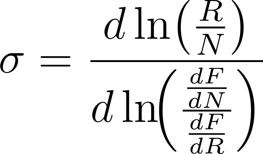
It tells us, at a given combination of inputs R, and N, how they can be traded off infinitesimally while maintaining a constant output. Crucially, it is a local statistic—it need not be constant across R and N, and there is little reason to assume it is. Economists often use CES production functions to avoid this issue but rarely consider shocks of the magnitude Barnett (2025) contemplates. To understand why assuming this local statistic remains constant at all scales can be dangerous, consider the following extension.
The aggregate CES production function economy is represented in Figure 1 (left). Final output (the node c) is a direct CES combination of the two factor inputs. Now look at the extended economy on the right: here, final output (still the node c) is a CES combination of the output of two firms (a – accountants and b – bricklayers). These two firms are each CES combinations of the two primary inputs R and N . Naturally, the bricklaying firm uses more non-remote labour, while the accounting firm uses more remote labour; however, both firms use at least some of each.
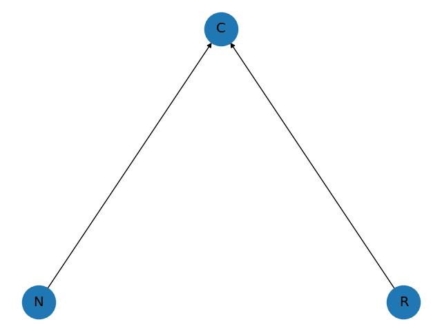 | 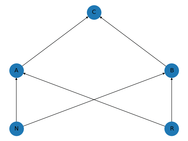 |
| Figure 1: (simple) In the simple model, the consumer goods producing firm (C) at the top is buying off each of the two factors (R, N ). | Figure 1 (continued): (extended) In the extended model, the consumer goods producing firm c combines outputs of accounting a and bricklaying b, each using both factors (R and N ). |
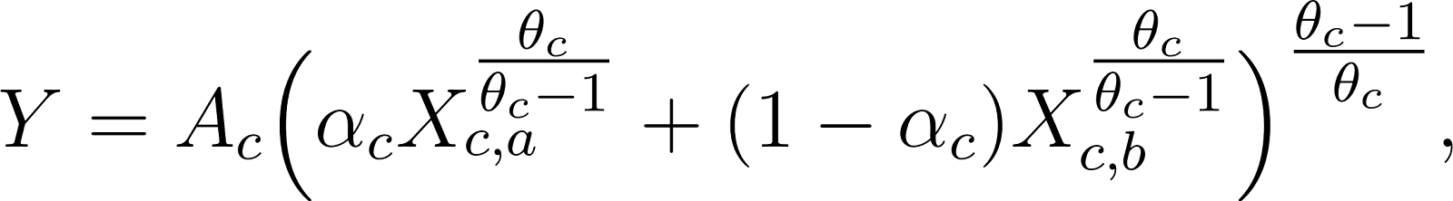
The production function for the simple economy is the two-input CES equation:
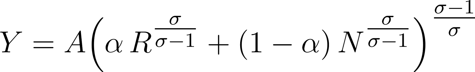
while the production function for the extended model can also be written explicitly as the nested CES function:
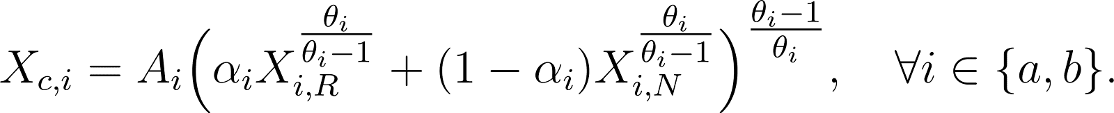
See Table 1 for a definition of each variable and parameter in Equations (1), (2), and (3).
| Table 2 | Description |
| Y | Total output |
| A, AC, Ai | Productivity (TFP) parameters |
| Share parameters controlling input weights | |
| Aggregate elasticity of substitution | |
| Elasticities of substitution for the consumer firm and the ith intermediate firm
|
| R, N | Quantities of remote (R) and non-remote (N ) tasks |
Inputs demanded by the consumer-goods producer (c) from sectors a and b, which equals their entire output | |
| Factor inputs for producer i sourced from R and N |
In the simple model, the eos between R and N is clearly a parameter, σ, which can be set freely. In the extended model, the aggregate eos between R and N is instead a weighted average of the micro-elasticities , where the weights are endogenously determined by the quantities of R and N.[4] For example, consider each of the following parametrisations of the extended model in Table 2.[5] The first 3 columns all start with aggregate eos close to 10 - and only otherwise differ in the eos for the intermediate firms . Parameter set 1 is equivalent to the simple model with a constant σ, as any weighted average of = 10 and = 10 is obviously 10, but σ is not constant for Parameter sets 2 and 3.
| Param set 1 | Param set 2 | Param set 3 | Param set 4 | |
| 0.34 | 0.34 | 0.34 | 0.34 | |
| 0.99, 0.01 | 0.99, 0.01 | 0.99, 0.01 | 0.75, 0.25 | |
| 10 | 10 | 10 | 44 | |
| 10 | 0.25 | 0.01 | 0.01 | |
Initial | 10 | 9.56 | 9.56 | 10.14 |
| Table 2: Comparison of four parametrizations. All imply an initial factor share for R matching 0.34 as in Barnett (2025). |
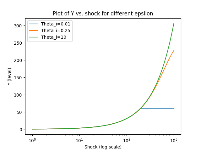
| Figure 2: A plot of Y against increases in R. Note all three behave similarly initially - but very differently by the time R is 1000x its initial level. |
To see how the global behaviour of Parameter sets 1, 2, and 3 differs, consider Figure 2. It shows how Y (initially normalised to 1) changes under different increases in R (also initially normalised to 1), for the three values ∈ {10, 0.25, 0.01}. The green line (
= 10) collapses the weighted average between
and
that defines to 10, making the model effectively identical to the aggregate production function. By contrast, the other two lines ( ∈ {0.25, 0.01}) initially show the same explosive growth but eventually hit bottlenecks.
Intuitively, as becomes smaller, any increase in R leads both the accounting and bricklaying firms to spend larger proportions of their budgets on N. Ever-lower prices of R thus have a reduced pass-through to final output. This occurs despite the fact that the final-output-producing firm c has a very substitutable elasticity,
= 10, and despite the fact this high substitutability initially dominates the aggregate eos.
To see this, look at Figure 3. It plots the aggregate eos between R and N as R increases, for the same values ∈ {10, 0.25, 0.01}. The bottlenecks are evident: both ∈ {0.25, 0.01} start out near 10 but eventually fall below 1 as R increases and
.
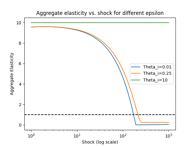
Figure 3: A plot of σ against R as R increases for different values of θi, dashed line is σ = 1. |
Of course, even the drastic case of = 0.01 in Figure 2 still results in a 50x increase in Y . This occurs because almost all factor inputs are reallocated to accounting, which is more efficient given the lower remote-work prices induced by a higher supply. However, we can set up a model with an initial aggregate eos σ ≈ 10 and an initial remote-work factor share of 0.34 (just as in Barnett (2025)) that does not yield such a large increase. Consider Parameter Set 4 in Table 2. Figure 4 shows the resulting aggregate output effects: despite an initial σ > 10, output is quickly bottlenecked at about 2.3x its initial level.
This model is highly stylized; real production chains are far more complex. For example, see Figure 2 of Carvalho (2014) for the US input-output network in 2002. Studying these networks—the macroeconomic consequences of their structure and the variations in elasticities across them—remains a highly active area of research (for example, see Baqaee and Rubbo (2023)). However, I believe there is strong evidence that we are moving closer to a world in which bottlenecks will arise. For instance, consider the benchmark calibration in the highly influential Baqaee and Farhi (2019). They suggest an eos of 0.9 for consumers across the industries they purchase from, an eos of 0.5 between primary factors and intermediate inputs, and an eos of 0.001 between intermediate inputs. While these elasticities are notoriously difficult to identify from data if these figures are even close to correct,[6] we would expect to be quickly bottlenecked by non-remote tasks.
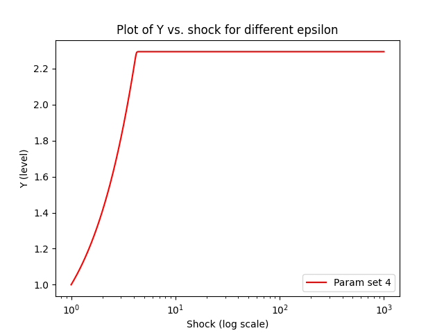
| Figure 4: A plot of Y against R as R increases initialized for parameter set 4. |
Empirics
The estimation of the current eos in Barnett (2025) behind the optimistic claim of σ = 10 has serious endogeneity issues, while the pessimistic σ = 0.5 is not particularly well justified.
Endogeneity of the optimistic case
Barnett (2025) fits an aggregate CES function like (1) to aggregate US data from 2008 onward. He takes the time series of Y, R, and N and finds constants A, α, and σ that best fit the data, estimating σ ≈ 12. Most co-variation in R and N during this period took place during COVID-19 when about one-third of the workforce switched to online work. There are several problems with extrapolating from these trends to estimate σ, all of which tend to bias the estimate upward. First, tasks that moved online were likely those easiest to complete remotely. Therefore, this shift does not reveal much about the substitutability of tasks that could not be done from home with those that were. Second, the historic US government stimulus to stabilize output during COVID-19 is not accounted for in Barnett’s analysis.
The pessimistic case is not a good lower-bound
For the “pessimistic” case (σ = 0.5), Barnett (2025) cites Anand et al. (2015). The cited paper investigates optimal inflation-targeting in developing countries when consumers may be close to the subsistence level of food intake. As such, they need a number that specifies consumer substitution behaviour in the face of changing food prices. They take a guess at 0.34-0.6 (depending on how they include the food subsistence level), but this doesn’t seem to be backed by solid estimates so much as intuitions. Moreover, empirical studies of production eos often find values far below 0.5, as noted in Section 2. For example, when examining how US sectors purchase intermediate inputs from one another, Atalay (2017) (a common benchmark in the literature) reports estimates much closer to zero. Therefore, I see no compelling basis for treating 0.5 as the lower bound for the current elasticity between remote and non-remote tasks at the aggregate level. Unsurprisingly, if we believe σ < 0.5 is more plausible, then increases in output (Y) derived solely from scaling up one input (R) can shrink dramatically.
Finally, and less crucially for the modelling approach, when setting α, one must decide how tasks are paid in reality. Wages are set by occupation, not by task, yet Barnett (2025) appears to assume all tasks have the same value, which is a strong assumption. For comparison, Acemoglu (2024) takes a different approach (see footnote 24). Barnett (2025) also compares estimates to Dingel and Neiman (2020), noting that many AI-automatable tasks currently earn higher-than-average wages. Accounting for that would likely raise α from 0.34 to something higher. Even a modest increase in α can have notable effects on at what level of output a bottleneck is hit.
Conclusion
Given the concerns raised above, I will focus on the research directions I believe are most critical. First, less emphasis should be placed on the current aggregate elasticities of substitution. Instead, those studying extremely large shocks should take a holistic view of production, investigating where bottlenecks may appear and how quickly they can become significant at the aggregate level. I am planning on writing a post on this soon. Second, if you believe AI will excel at certain economically important tasks well before it becomes broadly capable across all tasks, measuring the elasticity of substitution between these sets of tasks—especially at a more disaggregated level—is crucial. Along these lines, the idea of using COVID-19 as a natural experiment is promising, and I would be eager to see a more formal attempt at estimation.
Regarding the movement of existing workers from remote tasks to non-remote tasks once the former is automated, Barnett has informed me that his post will soon include variation in how extensively this is allowed. This consideration is vital in scenarios where bottlenecks arise quickly. Because CES functions exhibit constant returns to scale (homogeneity of degree one), the ability for workers to shift into N can raise the level of any bottleneck. Consequently, if bottlenecks are likely to emerge rapidly, further research into how easily workers can reallocate when their tasks or occupations are automated becomes essential.
Update log:
18/03/25: Fixed typos.
19/03/25: Fixed table 2 - previously said but only listed values. Now it lists and separately.
- ^
I would like to thank Eric Olav Chen, Rishane Dassanayake, Zach Mazlish and Sami Petersen for looking over drafts of this. I would also like to the thank, Luzia Bruckamp, Jojo Lee, Andrei Potlogea and Philip Trammell for useful points and conversations. Finally, I want to thank Matthew Barnett for posting his code and being fast and gracious in responding to emails. Code to generate Fig 2,3,4 are here. The method is Euler's using first derivative changes in factor shares as derived in Baqaee and Farhi (2019). They explain a very similar method more precisely on a more complicated model in Baqaee and Farhi (2024).
- ^
Barnett's GDP-increase graphs at the time of me posting this are outdated, still relying on an initialization error. When I pointed this out he quickly updated and got new graphs which should be in his post soon.
- ^
A draft version of this post also pointed out the last footnotes coding issue which is now being fixed.
- ^
See equation (1) of the technical note, the result is from Baqaee and Farhi (2019)
- ^
In each, we normalize initial levels Y=R=N=A_c=A_i=1, pushing all initial level differences into the shares , this is a standard trick with CES
- ^
Assuming we are not in a world where every occupation can seamlessly substitute its tasks with remote work at the micro level -Some
examples include cleaners, surgeons, and firefighters.