Uncertainty, Structure, and Optimal Integration
The EA community and Future Fund are running a risk in wasting good analysis of propositions when considering long-term predictions that entail complex, compounding uncertainties. Specifically, by ignoring or over-simplifying the complex ways our propositions interrelate (i.e., how they are “structured”), we stand to make substantial errors in our predictions. Moreover, the failure to appropriately “unpack” the structure behind our propositions risks substantial inefficiency in our focus of which uncertainties (whether they be based on a lack of information, or substantive disagreement) are more critical to resolve.
In Sections 1 and 2 I provide a primer to the uninitiated on the nature and importance of unpacking and disentangling the uncertain propositions that comprise our prediction problems.
In Sections 3 and 4 I lay out my analytical approach that seeks to capture and resolve these issues. I provide a fully worked through, illustrative decomposition of the misaligned AI X-Risk prediction problem, using a combination of Bayesian Network modelling and simulation techniques. My intent is to illustrate this analytical approach as a viable framework for a) making arguments and assumptions explicit and quantifiable in a unified manner, b) drawing mathematically optimal inferences (i.e., predictions) even in the face of multi-layered uncertainties, and c) laying the foundations for accessible computational methods that will assist further research. My assumptions and propositions within the model are predominantly grounded in extant estimates and analyses drawn from AI experts and fellow contributors. However, I highlight a number of previously overlooked or underspecified propositions and conditional probabilities that affect our predictions, but have previously remained hidden.
In Section 5 I step through the results of my analysis. Among them, I show that once structural disentanglement is taken into account, under reasonable, informed assumptions, the P(Misaligned AGI X-Risk) by 2070 is 1.68% (+/- 1.25%), rising to 6.53% (+/- 4.32%) by 2100. Though if we wish to assume an AGI has been built by 2070 (i.e., P(Misaligned AGI X-Risk|AGI)), then this rises further to 5.32% (+/- 3.42%) by 2070, and 11.22% (+/- 6.86%) by 2100. I additionally provide predictions for AGI build likelihoods across the target time-horizons.
Finally, in Section 6 I describe a quantitatively assisted path forward for further inquiry that is both viable and accessible. I outline how the analytical approach laid out here can be built upon; both enriching, and being enriched by existing lines of research into AI X-Risk.
1 - A Reasoning Under Uncertainty Perspective
Predicting the future existential risk due to a misaligned AGI is not only an important problem in and of itself, but is also useful as being illustrative of a class of problem. Prediction problems like this – much like any reasoning under uncertainty endeavour – require:
1) The acquisition of relevant arguments, assumptions, and propositions,
2) The estimation of the uncertainty surrounding them, and finally
3) Their integration into a coherent whole.
Substantial work has been done on the acquisition of relevant arguments in recent years (even just a cursory search of this forum reveals >400 posts on “AI Risk” at time of writing, dating back 6 years). These cover a wide array of topics such as AI build likelihoods and timelines, relevant AI properties/functions, paths to catastrophe, and risk countermeasures, just to name a few. Work like this - the acquisition of relevant arguments – is invaluable. Without such work, it would be as if we are trying to build a telescope without any components.
This post does not focus on the acquisition of arguments. I am not an expert on AI. I am, however, an expert on modelling complex inference problems. This post focuses on a way to integrate those acquired arguments to minimise the risk of error. Put another way, I design telescopes. The value of understanding good telescope design is not just in getting a clearer picture of what we wish to look at. It is far wider than this. The more one learns about how pieces should be arranged, the more one sheds light on which components are more important, and which are less so; which components need refinement to be fit for purpose; and which components we did not even realise we were missing.
As has been noted in the AI Prize Announcement and in advice on reporting here, explicit probabilities (i.e., estimation) are critical to reasoning transparency. They allow us to express degrees of confidence in a unified manner, lowering the risks of inadvertent, unhelpful translation error (e.g., what I mean when I say “X is likely” may be quite different from what you interpret). Moreover, explicit probabilities are critical in laying the groundwork for computational methods. Analyses such as Carlsmith (2021), responses to Carlsmith, Cotra (2020), and Davidson (2021), among others, have taken important steps in providing various estimates on the probability of various propositions (e.g., the likelihood of an AGI being built by a given year). However, as noted within Carlsmith’s own work (Carlsmith, 2021, Section 8), attempts to accurately integrate these estimates exposes two centrally important, but easily overlooked reasoning errors. These reasoning errors - when ignored - can lead to wildly overconfident predictions (as I will show). These errors are:
1) Oversimplifying Structure. Although the multiplication of probabilities attached to propositions is nominally a Bayesian way of integrating (conditional) probabilities (i.e., the application of a chain rule), it implicitly assumes a lot about the way uncertainty is structured. I discuss this in more detail below, but the most obvious assumption is that of unitary causation – a chain of probabilities implies a singular path of cause (or “parent proposition”) and effect (“offspring proposition”). Reality is far messier, with common causes of multiple effects, effects with multiple potential causes, and myriad combinations thereof. Simply put, this fundamentally changes the maths and risks substantial overconfidence in estimates derived from inadequately structured integrations.
2) Failing to “Unpack” Propositions. In relation to the first, there is recognition that an estimate attached to a proposition may in fact be covering hidden, unquantified parent propositions. For example, in arriving at an estimate of an X-Event caused by a misaligned AGI (P(X-Event|AGI)), one of my propositions may be the probability of an AGI being built successfully (P(AGI)). However, what is omitted from my estimate of P(AGI) are the propositions (i.e., assumptions) I have invoked (e.g., the likelihood of a build being computationally feasible; there being a viable AI design; there being sufficient incentive for completing a successful build). Without explicit estimates provided for these parent propositions, we not only risk introducing error to the overall calculation, but we are also not adhering to principles of transparency, making it harder to reach clear consensus on points of disagreement.
In this post I will demonstrate an analytical approach that directly addresses these problems. In so doing, I will outline how this approach:
- Provides useful structure to a complex problem.
- Disentangles compounding levels of uncertainty.
- Facilitates the move towards more exhaustive, transparent estimation of uncertainties surrounding propositions.
- Demonstrates optimal (i.e., inaccuracy minimization via Bayesian inference) integration across these structured uncertainties.
- Creates a computational method that can enhance the acquisition process; helping us see which propositions are more impactful to the question at hand, and therefore which areas should we invest more time in resolving remaining uncertainty/discordancy.
The model I create in the process serves as an example of a more accurate, transparent method of integrating what we know to make better predictions. To understand why this is the case, I provide a primer on why failures to appropriately understand and account for reasoning structure can systematically lead our predictions astray. Readers already familiar with the relationship between reasoning structure and reasoning errors should feel free to skip to Section 3.
2 - A Primer on Disentanglement[1]
There are myriad factors that make predicting long-term risk difficult. Ultimately, these stem from the different sources and implications of uncertainty types. For example, at the highest level we have uncertainty stemming from unknown unknowns (e.g., we do not know which arguments we have not yet made); this impacts the accuracy of our (reasoning) models, but is generally something harder to quantify meaningfully.
We then also have uncertainties that stem from known unknowns, which covers both empirical sources, such as incomplete data, measurement error, and instrument reliability; as well as more subjective bases, such as degrees of belief, and disagreement (e.g., community estimates diverging substantively regarding the likelihood of a proposition). Often, we tend to ignore some or all of these sources of uncertainty, either at worst by being “selective” (whether purposefully or not) in our supportive arguments and conclusions, or at best by trying to “summarise” across the uncertainties via a point estimate (i.e., a 1st order probability: “I believe there to be an X% probability that Y will happen.”). The latter of course is an important step towards reasoning transparency, but much remains to be desired.
For instance, let us consider the impact of disagreement in our probability estimates for a proposition. As disagreement increases (see examples here and here), so too does the 2nd order probability (see e.g., Baron, 1987) surrounding the proposition. For example, if we compare two hypothetical cases; one in which 100 experts have all given probability estimates for the probability of an AGI being built by 2070 between 48% and 52%, and another in which they gave estimates between 20% and 80%. In both cases, our overall (average) point estimate for P(AGI built by 2070) is 50%, but we can see how in the former case, we can be much more confident of that 50% as individual estimates lie +/-2% either side, than we can in the latter case, where there is much more substantial disagreement with individual estimates lying +/-30% either side.
This form of uncertainty is important, but difficult to deal with without computational assistance. As we consider how to integrate multiple propositions to arrive at a conclusion, these uncertainties in fact compound potential errors. Fortunately, as we start to disentangle the reasoning structure that underpins and connects our propositions (the central purpose of the analytical approach laid out in this post), we can not only gain more transparency and insights behind why we are disagreeing (via structurally “unpacking” a proposition), but we can avoid compounding errors in our integration. To return to our telescope analogy: If we are trying to identify something far away (our prediction), and we have a handful of lenses (our collection of propositions), we are far more likely to end up with a blurry image (and thus a mistaken identification) if we do not know how to arrange our lenses correctly. Once we know the principles for how the parts should be arranged, we are then also much more able to discern which lenses may be causing problems (i.e., once we know the correct design, we also know how clear the image should be).
Where does this leave us? First, we have multiple sources of uncertainty when we try to make predictions. Second, how these uncertainties affect our predictions when we must integrate across multiple propositions is complex, and consequently carries a high risk of error. So, if we wish to make better predictions, we must understand how to capture and deal with this complexity. To achieve this, we must next understand how uncertainties can be disentangled (or “partitioned”) using reasoning structure:
2.1 - Structure
Understanding how a proposition relates to and interacts with others is perhaps one of the hardest, but most critical parts of correctly integrating arguments to arrive at a more accurate prediction.
2.1.1 - Conditionals and Chains
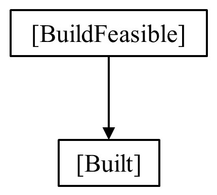
Let us begin with the difference between the probability of a proposition being true, and the probability of a proposition being true conditional on something else (e.g., a parent proposition) being true. To help explain this, and all forms of structural disentanglement outlined in this section, I will use a toy example version of the likelihood of an AGI being built – this is meant to be purely illustrative at this stage, so do not worry about specific estimates.
First, let us assume the probability of an AGI being built (P(Built)) at least in part depends on the probability of it being technically feasible and affordable to construct an AGI (P(BuildFeasible)). Now, let us assign a probability – say 30% - to the proposition of an AGI build being feasible by a chosen point in time (i.e., P(BuildFeasible) = 30%). This is not the same as the probability of an AGI actually being built (i.e., P(Built)). This latter probability is only inferable, via the conditional probability of a successful build, given its feasibility. For instance, we may assume that if an AGI build is feasible, then there is a high probability of an AGI getting built – say 80% (i.e., P(Built|BuildFeasible) = 80%). We can also assume that if an AGI build it not feasible, then an AGI cannot be built (i.e., P(Built|¬BuildFeasible) = 0). We can see the outcome of this integration via Bayesian Inference below (note: for a more thorough read than this short example, see this post by Eliezer Yudkowsky):
Given our assumptions above, this translates to:
Although this example is simplistic, it gets across two important aspects of structural disentanglement:
- It exposes potential sources of error in informal reasoning. Some potential errors include (but are not limited to):
- Base Rate Neglect: Ignoring base rate / prior information (in this example, this would be our parent proposition, P(BuildFeasible)). This can lead to gross overestimation. Here this would be assuming P(Built) = 80%, rather than the 24% we find when we properly structure the argument.
- Miss Rate Neglect: Although less relevant in this example, neglecting terms like P(Built|¬BuildFeasible) fails to account for “would this have occurred anyway, regardless of my parent proposition?” This failure can produce substantial over or underestimations of the likelihood of a proposition being true, as you are not fully accounting for the strength (how predictive/diagnostic) of the relationship between the two propositions.
- Put simply, the separation into terms forces us to scrutinise and incorporate a more complete set of uncertainties, reducing errors.
- The disentanglement allows us to better identify where we are disagreeing, and where we are less certain (e.g., our different P(Built) values are stemming from different assumptions regarding P(Built|BuildFeasible), whilst we mainly agree about P(BuildFeasible) itself). Though arguably trite in this example, this capability becomes increasingly needed the more complex the overall reasoning structure, as we will see.
We are starting to see how separating out structure supports more thorough and efficient acquisition (and consequently, estimation) of propositions.
So far, we have laid the groundwork for integrating across a causal chain, wherein we can multiply a chain of conditional probabilities together to reach a final proposition likelihood. This has been the method applied by Carlsmith (2021) and others when estimating AI X-Risk. Of course, when we start to consider uncertainties on each of these component probabilities, things get a lot trickier (see this excellent post on uncertainty analysis of the same causal chain by Froolow). Additionally, in modelling these arguments we must draw a line under “how far back” we wish to go: P(BuildFeasible) is itself conditional on other propositions, and so on backwards until we reach the Elysium of exhaustive, confirmed certainty. This of course is rarely possible, particularly in long-range prediction. Thus, we must elect to “cut off” the recursion at some point.
This is not where the story ends, as we have the obvious fact that one proposition may have more than one effect on other propositions, and itself be affected by more than one parent proposition. As we will see below, when we expand our understanding of reasoning structures to include this broader set of possibilities, the grave implications of ignoring this complexity for prediction accuracy will become evident – along with the rationale for the analytical approach outlined in this post that captures this complexity.
2.1.2 - Common Effects
Next, let us consider a proposition with more than one parent (known as a “collider”, or common effect). This is an extremely likely occurrence – rarely is it the case that unitary causation (i.e., one cause to one effect) is valid. For example, there are often enabling conditions, additional risk factors, catalysts, and so on. Each additional parent proposition results in a combinatorial explosion of the proposition that depends upon them.
To ground this in our example, let us reconsider it, but now add an additional influence on P(Build): the (human) incentive for AGI, P(Incentive):
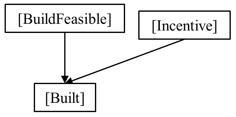
If we return to our original example, where P(BuildFeasible) = 30%, but now we assume that by this time, there will more likely than not be an incentive for an AGI (e.g., P(Incentive) = 60%). Further, we can now specify that if a build is feasible and there is incentive, there is a high likelihood of a successful build (e.g., P(Built│BuildFeasible,Incentive) = 90%), but if there is no incentive, this drops substantially (e.g., P(Built│BuildFeasible,Incentive) = 5%). Given we can again assume a successful build is impossible if the build is not feasible regardless of incentive, this gives us:
When we compare this ~17% to our previous calculation (where P(Built) = 24%), we can see how by failing to unpack and incorporate this additional parent (i.e., by keeping our incentives assumption hidden / unaccounted for), we are incurring a systematic error (in this case, overestimation). This is particularly critical when we consider that these errors can compound (i.e., our overestimate forms the basis of a further calculation, that itself could be an overestimation, increasing the overall inaccuracy).
More generally, we can also see that computational requirements have doubled. In fact, for each additional parent (as there can of course be more than two), we must increase the number of terms exponentially.[2] It is worth emphasising again here that these unpacked terms are still present in an informal analysis of these propositions – they are simply unspecified and their influence unaccounted.
In this way, we once again highlight the value of unpacking our assumptions and structuring them appropriately if we are to 1) reveal where we might be missing important information, and/or where our points of disagreement lie (assisting in both acquisition and estimation), but also critically 2) enable optimal integration.[3]
2.1.3 - Common Causes (and Dependence)
Finally, and to complete the picture, we must consider a parent proposition with multiple offspring propositions (known as a “fork”, or common cause). This is simple enough when we only care about each offspring proposition in isolation (i.e., we can multiply our conditionals, as we did for a chain).[4] However, how common causes fit into the bigger picture of our reasoning structure has substantial implications for the accuracy of our predictions.
For instance, what if a parent proposition for one part of my chain is also a parent to another part of my reasoning chain? Extending our previous example P(Incentive) may not only affect whether an AGI is successfully built (P(Built)), but also whether it will go on to be deployed within a target system (P(Deploy)).
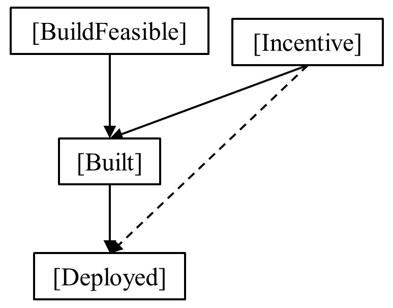
The influence this common cause is having on the overall reasoning structure (and therefore our predictions) is often described as dependence. Essentially, propositions considered independent carry more weight than when they share a (partial) basis. If I am not explicitly accounting for the fact some of my propositions share the same parent, then I am not factoring in that there is some redundancy in my reasoning. Instead of subjecting you to even more maths (though see Koller & Friedman, 2009; Pearl, 1988; Schum, 1994; for full mathematical treatments) I will illustrate with a quote attributed to Abraham Lincoln:
“Surely, Mr. Lincoln,” said I, “that is a strong corroboration of the news I bring you.” He smiled and shook his head. “That is exactly why I was about you about names. If different persons, not knowing of each other’s work, have been pursuing separate clews that led to the same result, why then it shows there may be something in it. But if this is only the same story, filtered through two channels, and reaching me in two ways, then that don’t make it any stronger. Don’t you see?”
William Seward (1877)
Setting to one side the implications this has for how much weight we should assign aggregation/consensus across AI experts (there is an entire separate post that could be written on potential community overconfidence in that regard), we can see the implication of Abe’s words for our own prediction efforts: If our prediction relies upon seemingly separate propositions – but these propositions in fact draw their strength from the same parent(s), then we are likely to be overconfident in our conclusions.
Along with exposing redundancy, disentangling these common causes in our reasoning structures also helps us avoid logical inconsistency in our reasoning – for example, a shared parent that makes one offspring proposition more likely, but makes another less likely, can cancel out the impact our two offspring propositions would have had on our prediction.
Once more, I will trumpet my standard refrain about how this disentangling is necessary and helpful for more exhaustive acquisition and estimation, and essential to accurate integration. In addition, I note that factoring in these sorts of structures can expose where propositions within our reasoning problem are more sensitive to changes in our parameters. If multiple parts of my chain actually rely on the same parent proposition, then my assumptions regarding the parent proposition (including the uncertainty that surrounds it) will have more impact on the overall reasoning structure and my predictions (ceteris paribus) than my assumptions regarding one of its offspring.[5]
So, we have now covered the three core reasoning sub-structures (chains, common causes, and common effects), and how failure to account for them can lead to error. Critically, all reasoning under uncertainty problems are built using these three core sub-structures, just using various combinations. Predicting misaligned AI X-Risk is no different. I will again emphasise here that these structural complexities are part of the prediction problem, regardless of whether you represent them within a model.
To return to our telescope metaphor: At this point I have sought to highlight the importance of appropriately combining our components by showing that without appropriate assembly, the image we are trying to see will be hard to interpret accurately. Extending the metaphor slightly, the further we are trying to see, the more substantial the components (propositions) we are likely to invoke, and thus the stronger the imperative to arrange those components correctly. Slight misalignment in a set of binoculars will limit the image quality, but misalignment in the James Webb Space telescope would render it useless – given how far it is trying to see.
Where does this leave us? Fortunately, there are computational approaches that allow us to capture and navigate this complexity. Here I demonstrate one.
3 - Current Approach
My analytical approach here has two interrelated components:
First, I have constructed a Bayesian Network model for predicting misaligned AI X-Risk. This model disentangles how a number of core propositions relate to one another, and in so doing accounts for the potential pitfalls and errors described in Section 2. Further, this disentanglement exposes a number of relevant conditional probabilities that at time of writing have not received much consideration when we discuss AI X-Risk. In this way, the model opens the door for improving acquisition and estimation goals by increasing the necessary transparency of our reasoning.
Perhaps most critically of all, the model incorporates a probability calculus that enables optimal integration across the complex pattern of inferences. Once more I will emphasise that this complexity is inherent within the prediction problem, whether we choose to capture it or ignore it. Furthermore, the way the model is structured draws from other domains of reasoning-under-uncertainty to highlight several useful ways of breaking down the AI X-Risk prediction problem.
Second, surrounding the Bayesian Network model I have built a simulation “wrapper”. This wrapper selects parameters for the model (e.g., our chosen conditional probabilities), runs the model with those parameters, recording the predictions that model makes, and then begins again with a new set of inputs. We can think of it like this: The Bayesian Network is the telescope design, and the simulation wrapper is a conveyor belt swapping in new lenses and recording the picture. This enables me to do several things:
- I can see how model predictions change for each year moving forward as input propositions are predicted to change through time (layer 1). This allows me to ask an expanded set of questions, and ties the temporal dimension into the coherence of the analytical approach. Put another way, we can explicitly track how predictions change through time, generated via the same, consistent calculus and structure.
- Second, for every year, I run repeated versions of the model, where parameter inputs are drawn from a distribution, rather than fixed to a single number (layer 2). This stochastic sampling process enables me to incorporate the 2nd order probability that affects our estimates for each proposition (see Section 2 for discussion on the way unknowns and disagreements affect our estimates). In this way, we can determine how much uncertainty surrounds our generated predictions.
3.1 - Bayesian Network
Simply put, a Bayesian Network is an argument map with some maths underpinning it.
More concretely, Bayesian Networks have a graphical representation, known as a Directed Acyclic Graph (DAG), where the relationships (arrows) between each variable (in our case, these are our propositions) are conditional probabilities (Pearl, 1988). Variables without any parents (i.e., no arrows flowing into them) are described by a “prior” probability at the input stage. In other words, we are fixing an initial probability based on our assumptions. This differs from variables with parents, as these can only initially be described by a set of conditional probabilities (see Section 2.1); the likelihood of that variable being true is always the product of inference. Crucially, this inference process is Bayesian, and may be considered optimal in the sense that it minimises inaccuracy (see e.g., Pettigrew, 2016).

In the model structure shown above, variables (our propositions) are labelled using [square braces], this is to distinguish a variables state (here these states are True/False, though other states are possible) as either true [X] or false [¬X]. This is distinct from the probability of a proposition being true P(X) or false P(¬X). I will unpack each of these variables and their connections in turn in the model description below. Suffice to say that inferences flow from parentless propositions (or premises) {[SSu], [SBl], [De], [BFe], [Op]}, through an intermediary layer of inferred (read: conditional) propositions {[Po], [MAG], [CCo], [Bu], [In]}, which in turn are parents to the central inferred proposition of interest {[AIX]}.
We can use the network to “read off” updated inferences about each of our propositions simultaneously, and can even assess the impact of making particular assumptions/observations. For example, if we wish to assume an AI has been built (rather than leave it as an inferred probability), we can set that proposition to true, and see how this changes the pattern of inferences in the rest of the model.
3.1.1 - Sub-structures
Though we can see already from Fig. 1 that the network is comprised of the reasoning structures outlined in Section 2 (e.g., [De] -> [CCo] -> [AIX] is a chain, whilst [De] is also the common cause of several propositions, that in turn are also common effects of other parent propositions, and so on…), I felt it prudent to further classify these propositions – particularly in how they relate to the central proposition of interest.
In asking “will a misaligned AGI cause an X-event”, we are essentially asking how likely is it an “agent” (a misaligned AGI) will commit an “act” (an X-Event). This is the prediction equivalent of the diagnostic question: “how likely is it [agent] committed [action]?”. For this reason, there are similarities between our question and reasoning under uncertainty in legal settings, wherein determining guilt can be broken down into separate sub-structures (see e.g., Lagnado et al., 2013), each of which plays a role when assessing probable guilt. In part as useful structural metaphor for signposting my reasoning, I use and extend these here, to arrive at the following categories of proposition:
Means: Propositions relating to the question of whether an AGI will have the tools/potency to enact an X-Event (in a murder case, this would be possessing the murder weapon).
Motive: Propositions relating to the question of whether an AGI will intend to enact an X-Event (this does not mean through maliciousness necessarily, rather through misalignment – accidental or otherwise).
Opportunity: Propositions relating to the question of whether an AGI will have the necessary access to enact an X-Event.
[Additional] Existence: As it does not exist yet, we also must consider propositions relating to the creation of an AGI as a necessary enabling condition.
[Additional] Enabler Incentive: Similarly, as an entity that we can assume at least initially requires external assistance (even if this is just to create the AGI), we should also consider propositions regarding human (as enabler) incentives.
Although the above has proven useful to me in my structuring of the model, it may prove a useful classification for others when considering how to direct research and collate arguments. For instance, it may be that means, motive, and existence have received far more thorough treatment or reached firmer consensus than opportunity and incentives. The classification is also useful for basic sensitivity analysis in future – informing us about which categories are more impactful to our predictions.
3.2 - Simulation "Wrapper"
The simulation wrapper is essentially a series of loops that generate multiple independent Bayesian Network model runs. These runs differ in the input parameters provided to the model, whilst the structure of the model remains constant.
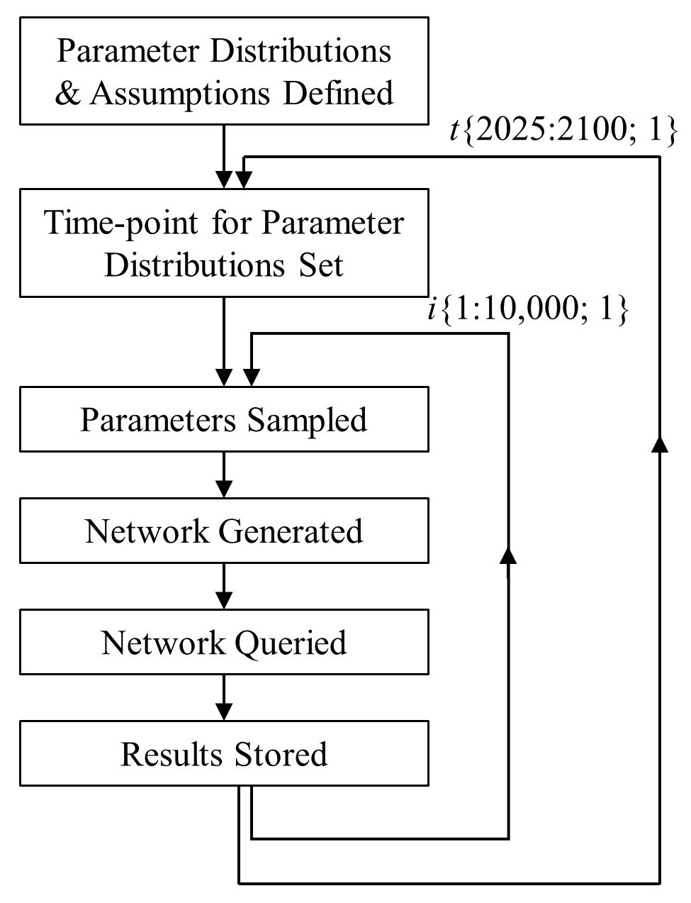
The first “layer” allows us to investigate how inferences change as inputs change over time, wherein I specify a time-series for each relevant parameter. In this way, how the model outputs (i.e., the predictive inferences we are “reading off” the model) change over time can be recorded and assessed. This is a critical component, given the importance of the temporal dimension to many of these sorts of prediction problems. I note here that although it is possible to incorporate inter-temporal dynamics (e.g., success in a previous year in one part of the problem changes the dynamics in other parts), in this initial version of the model these are set to one side.
The second “layer” occurs within each time-point, and entails repeated stochastic sampling (10,000 samples per time-point) from specified distributions (any distribution shape can be specified independently for each parameter, including normal, beta-geometric, see e.g., this recent post by Froolow on importance of these decisions). This allows us to capture second order uncertainty regarding our model inputs.
Taken together, the simulation wrapper allows us to not only see how model predictions change over time, but also how uncertainties at input stages translate to uncertainties around those predictions, which can often be highly unintuitive.
3.3 - Approach Summary
Before summarising the approach, I will once again emphasise that the complexity laid out above (the role of conditional probabilities and reasoning structure, the role of time, and the role of 2nd order uncertainty) is still there in our prediction problems, whether we represent it within a model, or not. If we do not represent it formally, we are simply unaware of the nature of the compounding errors we are making, and thus we are prone to overconfidence in our conclusions.
Through the analytical approach laid out here, we can represent and account for this complexity by making it explicit; in turn allowing us to integrate optimally, given our explicitly stated assumptions. I argue that at this stage in the investigative process – where methods for accurate integration are particularly required, this has great value. This approach sets us on the path to learning which unknowns are most critical, such that we can start to seek agreement on shared assumptions/parameters – or simply see the impact of our disagreement.
In the model description laid out below, I have no doubt that some of my assumptions will provoke disagreement – as I have mentioned, I am not an expert on AI. However, wherever possible I have made use of existing arguments and estimates, and I incorporate 2nd order uncertainty where there appears to be disagreement. Critically, I am feeding these existing arguments into an analytical approach that captures the complexity that surrounds them, enforcing much needed exhaustiveness and transparency, and enabling accurate integration.
4 - Model Description
The Bayesian Network model is written in R for now using the gRain package (Højsgaard, 2012); I have made all the code available here. Feel free to download it and run it yourself. I have done my best to indicate clearly within the code where different assumptions/parameters can be specified.
In this section I describe the model by stepping through each proposition in turn. This description begins with parentless propositions which have prior probabilities directly specified. I then build up the model description, beginning with the most immediate inferred propositions, on until all propositions (and how they relate to one another) have been explained. Usefully, a property of Bayesian Networks called a Markov blanket means we can understand an inferred proposition by knowing only its immediate parent propositions. This partitioning property allows us to build up the complete picture of the model by focussing on each piece in turn, without missing anything critical about the model as a whole.
4.1 - Terminology
AGI: Here I take this to mean an Artificial General Intelligence, such that it possesses sufficient features to enable concerns regarding goal misalignment and circumvention of control.
System: The system/context in which an AGI is implemented.
User/Implementer: The human(s) responsible for initial activation of the AGI within the system.
Parameter Uncertainty: Here described as +/- 1 standard deviation (SD). Of course, other measures are available.
4.2 - Prior/Parent Propositions
These are probabilities for parentless propositions, which where possible are drawn from existing analyses (notably Carlsmith, 2021; Cotra, 2020). As I have mentioned, although point estimate probabilities are an excellent step, it is important to represent the uncertainty surrounding them, as the way uncertainty propagates across the reasoning structure can often produce unintuitive effects (cf. Schum, 1994). In this way, provided point estimates are considered central tendencies in probability distributions of varying width (from which sample parameter values are drawn for model runs).
Given the question focus on the year 2070, and the consequent prior analyses also providing estimates based on this year, time series inputs trend towards them, following 3 basic assumptions:
- Uncertainties will grow over time (represented here as standard deviations, but other measures can be interchanged for reporting purposes).
- The trend that takes us from the current time-point to 2070 is expected to continue (i.e., I am not assuming there is something a priori “special” about the year 2070).
- Unless there is a strong reason to deviate, I will assume steady, continuous linear change in input parameters over time. This is to avoid smuggling additional assumptions, including assuming 2070 as a particular year of importance (e.g., as an inflection point in a sigmoid function). *Note: Other temporal functions are of course testable assumptions within the model, though I will note for the purposes of the 2070 question (and the estimates for that year originating in prior analyses, not my chosen function), this for now is immaterial.
4.2.1 - AGI Feasibility & Design Propositions
Probability of building an AGI build being feasible: P(BFe)
Proposition: Is an AGI feasible and affordable?
Assumptions Basis: The probability of there being sufficient, affordable computational capacity for the creation and maintenance of an AGI. Here, I am assuming this to mean the probability that the necessary resources (hardware, finances, etc.) are sufficient for the creation of an AGI. I note here that this proposition itself can be unpacked into subsidiary propositions, applying the current method recursively. However, for the sake of my own time constraints, I will not dig into this for now. Instead, I will seek to incorporate parameter values from existing analyses.
In general, the year-on-year probability is assumed to grow over time, and has been covered in analyses such as Cotra (2020). These analyses place the probability of sufficient computational capacity (read physical and financial feasibility) for an AGI by 2070 at 65%.
Detail/Function: Consequently, I assume this probability to continuously grow to reach 65% by 2070, and then continue growing at a similar rate beyond 2070. Further, I am attaching a growing uncertainty in this parameter the more distant the prediction, such that by 2070, this 65% probability has a +/- 14.16% uncertainty surrounding it. This range around the point estimate covers a broad range of estimates (approx. 50% - 80% within 1 SD), helping to encompass acknowledged variance in these estimates.
Probability of successful AGI Design: P(De)
Proposition: Is there a viable AGI design?
Assumptions & Basis: The probability of there being a viable AGI design that possesses the necessary capabilities for misalignment of goals and circumvention of human control, namely, as described by Carlsmith (2021), agentic planning and strategic awareness features. Again, and as laid out by Carlsmith, this proposition itself can be unpacked into subsidiary propositions. Although the method described here could be deployed to unpack and integrate this sub-proposition set, for now I will take the previously analysed composite. The specified year-on-year probability is assumed to grow over time, and has been well-covered in analyses such as Carlsmith (2021). This value is assumed to be married up with the same rate as the build feasibility [BFe] (i.e., 65% by 2070). However, to represent some of the disagreement and uncertainty on this proposition, uncertainty in this parameter is again built in.
Detail/Function: Consequently, I assume this probability to continuously grow to 65% by 2070, and then continue growing at a similar rate beyond 2070. Further, I am again attaching a growing uncertainty in this parameter the more distant the prediction, such that by 2070, this 65% probability has a +/- 14.16% uncertainty surrounding it. This range around the point estimate covers a broad range of estimates (approx. 50% - 80% within 1 SD), helping to again encompass acknowledged variance in these estimates.
4.2.2 - User and System Propositions
Probability of recognising harmful features of an AGI (i.e., the Opacity of the AGI): P(Op)
Proposition: How likely are we to recognise the potential threat characteristics / risks associated with an AGI implementation?
Assumptions & Basis: The probability of the AGI implementer/user having sufficient understanding of the full capabilities of the AGI (read: misaligned goal, control subversion capability, and sufficient power to commit and X-Event) has arguments that both increase and decrease it. For example, on the one hand the increasing complexity required to design and build an AGI is likely to increase the difficulty of recognising potential risks/threats, and notably if self-modification and improvement is assumed (e.g., Bostrom, 2014 Ch.6 on the link between recursive self-improvement and covert preparation potential). On the other hand, advances in the development of potential interrogative tools (for examples of interpretability improvement, see e.g., Olah, 2020; and Goh et al., 2021) and an increasing prevalence of blanket assumptions/weariness regarding potential (deleterious) AGI capabilities, may mitigate some of this increasing opacity. On balance I still assume it to become increasingly difficult to effectively understand an AGI regarding its potential risk, but attach a high degree of uncertainty on this assumption.
Detail/Function: For now, P(Op) is assumed to increase over time, such that by 2070 there is a 50% probability that the potential implementer/user of an AGI is no longer able to understand its full capabilities, with +/- 14.16% uncertainty surrounding it (again covering a broad range of potential estimates, from approx. 20% to 80% within 2 SD).
Probability of System being Susceptible to an AGI X-Event: P(SSu)

Proposition: How likely is the system in which an AGI is implemented to have sufficient “levers” for an enacting an X-Event?
Assumptions & Basis: The probability of the system being susceptible is a proposition that itself could be unpacked further with additional analysis and research. However, for now I note several important factors that are amalgamated to inform this proposition: First, there is consideration of which type of system an AGI will be implemented within (e.g., military, economic, scientific, commercial), and second, what the general connectedness of those systems may be – irrespective of initial implementation likelihood. If systems are sufficiently connected, then an AGI’s power stems from the use of that connectedness (e.g., in a highly connected system, an AGI originally implemented within a commercial system may make use of connections to power stations, logistical hubs, and so on).
In determining the estimate for this proposition, I note arguments have been made for a wide range of potential values. For example, there are arguments that our systems are already highly susceptible (with various mechanisms laid out in Carlsmith, 2021) – though I note this is not the same as whether they will be so in future. Alternatively, there are arguments that our systems will become increasingly connected/centralised (see e.g., globalisation and ICT trends; Friedman et al., 2005), leading to a rising probability of susceptibility. Then again, there are arguments that other shocks, “warning shots”, and risk factors may lead to increased partitioning and segmentation (e.g., along national boundaries; see e.g., border closure in response to contagion events; national protectionism responses to recent food crises), which may in turn decrease the potential (X-Event) potency of an AGI application. Along these lines, I also note separate instantiations of AGIs via competing national interests (see e.g., Bostrom, 2014, for discussion of “multipolar” scenarios) are immensely hard to predict their overall effect (e.g., succeeding or failing to recognise warning signs in other nations).
Consequently, I highly recommend this area of inquiry for further research in shoring up this proposition.
Detail/Function: For now, P(SSu) is assumed to increase, such that by 2070 there is a probability of 20% that the system within which an AGI is implemented is vulnerable to an X-Event action by an AI, with a +/- 14.16% uncertainty surrounding it (allowing for estimates as high as 50% within 2 SD).
Probability of System Blindness: P(SBl)

Proposition: How likely is the human AGI user/implementer to understand the target system well enough to recognise possible misuse/goal misalignment/control subversion?
Assumptions & Basis: The probability of someone with the power to implement an AGI into a system knowing the relevant properties of the system itself (e.g., relevant safeguards, unintended vs intended uses). Similar to consideration of AGI feature transparency/opacity [Op], system vulnerability blindness is expected to increase over time. Using similar logic, this is based on trends regarding system complexity resulting in the potential AGI user/implementer being less and less likely to comprehend sufficiently the system they inhabit (note: System here can be more generalised – e.g., internet), and with particular regard to potential AGI “misuse”. But again, I note here that there are arguments that work to offset this trend. In particular, the development of potential interrogative tools and assistive technologies for things like vulnerability testing (for example, growth in cybersecurity tools and services has seen continued, rapid growth in response to increasing user awareness of their system vulnerabilities to rising threats), and the potential influence of increasing prevalence of blanket assumptions/awareness regarding potential system abuse, e.g., via previous “warning shots” and partial misalignment instances (see e.g., Carlsmith, 2021).
Detail/Function: For now, P(SBl) is assumed to increase over time, such that by 2070 there is a 40% probability that the potential implementer/user of an AGI does not understand the target system well enough to recognise possible misuse/goal misalignment/control subversion, with +/- 14.16% uncertainty surrounding it (again covering a broad range of potential estimates, from approx. 10% to 70% within 2 SD).
4.3 - Conditional / Inferred Propositions
These propositions are considered conditional, in that their likelihood of being true or false stems from the propositions that affect (read: cause) them. Each of these propositions requires the specification of the strengths of the relations between it and its parent propositions, specified using conditional probability tables (CPTs). These lay out explicitly the assumptions regarding how each parent proposition will affect this variable, in combination with every other parent proposition.
At the risk of belabouring a point here, I wish to make abundantly clear that the conditional probabilities outlined here are based on “if cause/premise A is TRUE, then there is a X% probability this effect B would also be TRUE” – which is not making any assessment of how likely cause/premise A is in the first place.
To avoid concerns of false precision, wherever possible I have attached uncertainties to each conditional probability, considered in the simulation process. Although time series trends could also be specified for each of these conditional probabilities as well (as was done for the prior/baseline input probabilities), for the sake of parsimony this is omitted for now.
Additionally, I have taken the liberty of colour-coding the conditional probabilities in my CPTs. Specifically, estimates in green are drawn from logic, and thus I feel are self-evidently quite solid. Estimates in yellow are informed by pre-existing analyses, but carry uncertainty given their novel application here. Estimates in orange are novel considerations that have not yet received thorough analysis and estimation by experts. Although I have generated what I believe to be plausible placeholders, these latter values are excellent candidates for further analysis. This helps demonstrate the value of this approach in enforcing exhaustiveness and transparency when we make our estimates.
4.3.1 - Motive
Probability of an AGI possessing a MisAligned Goal: P(MAG|SBl,De)

Proposition: How likely will the AI design lead to misaligned goals when implemented within the system?
Assumptions & Basis: The probability of a potential AGI design resulting in goal misalignment when implemented within a system (to deleterious effect) can be argued as a consequence of poor fit between the AGI design (i.e., its derivation of goals) and the context of its initial system of implementation. Here I am assuming the AGI design [De] (replete with features like agentic planning and strategic awareness) is highly likely to develop misaligned goals (again, see Carlsmith, 2021, for a recent analysis of the relationship between these features and misalignment goals).
However, this misalignment probability can also be influenced by the user/implementers understanding of the system/context intended for the AGI (i.e., [SBl]). Put another way, an implementer with excellent system awareness (i.e., [¬SBl]) might be able to lower the risk of misalignment by changing the system to re-define goals a priori, for instance by adequately attending to and making use of potential “warning shots” and possible previous partial failures (see Carlsmith, 2021). Conversely, if system users are blind to the nature of their system/context, then this increases the likelihood of an AGI successfully operating with a misaligned goal. When we consider this assumption in relation to the larger question of an AGI X-Event, we can consider the misaligned goal as equivalent to motive in a legal case.
Detail/Function: The inference function here is primarily a logic gate: a misalignment risk cannot occur if there is not a viable AGI design [¬De]. However, if there is a viable AI design, then it is highly likely (60-80%) that a misalignment will occur, with system blindness [SBl] pushing this towards the upper end of this likelihood (80%, +/- 10%), versus accurate system knowledge [¬SBl] lowering this slightly (60%, +/- 10%). In this way, system awareness may make some difference to misalignment risk, but this risk is primarily dictated by the AGI design.
| Conditional[6] | MAG | ¬MAG | Uncertainty (SD) |
| P(MAG|De,SBl) | 80% | 20% | +/-10% |
| P(MAG|De,¬SBl) | 60% | 40% | +/-10% |
| P(MAG|¬De,SBl) | 0% | 100% | 0 |
| P(MAG|¬De,¬SBl) | 0% | 100% | 0 |
4.3.2 - Opportunity
Probability of an AGI Circumventing (human) Control: P(CCo|SBl,De)

Proposition: How likely will the AGI design lead to the capacity to circumvent human control within a system?
Assumptions & Basis: The probability of an AGI subverting existing control is conditional on the design of that AGI [De] incorporating necessary features for subversion (e.g., agentic planning, strategic awareness; see Carlsmith, 2021), and (again, to a lesser degree) the implementers understanding of the system/context intended for the AGI [i.e., SBl]. An implementer blind/ignorant of the risk of control circumvention increases the risk that an AGI will be unimpeded in circumventing control. Whilst if an implementer knows their target system well, they may be able to lower control circumvention risk (e.g., via a priori intervention, or external failsafe designs), as well as making use of potential “warning shot” partial failures from previous (minor) implementations. When we consider this assumption in relation to the larger question of an AGI X-Event, we can consider the capacity to circumvent control as equivalent to opportunity in a legal case.
Detail/Function: As with misalignment risk, the inference function here is also primarily a logic gate: a circumvention of control risk cannot occur if there is not a viable AGI design [¬De]. However, if there is a viable AGI design, then it is highly likely (60-80%) that circumvention will occur, with system blindness [SBl] pushing this towards the upper end of this likelihood (80%, +/- 10%), versus accurate system knowledge [¬SBl] lowering this slightly (60%, +/- 10%). In this way, system awareness may make some difference to circumvention of control risk, but this risk is primarily dictated by the AGI design.
| Conditional[6] | CCo | ¬CCo | Uncertainty (SD) |
| P(CCo|De,SBl) | 80% | 20% | +/- 10% |
| P(CCo|De,¬SBl) | 60% | 40% | +/- 10% |
| P(CCo|¬De,SBl) | 0% | 100% | 0 |
| P(CCo|¬De,¬SBl) | 0% | 100% | 0 |
4.3.3 - Means
Probability of an AGI having sufficient Power to cause an X-Event: P(Po|De,SSu)

Proposition: How likely will the designed AGI be able to cause an X-Event?
Assumptions & Basis: The probability of an AGI possessing sufficient power to cause an X-Event is conditional on both the design of the AGI [De] containing requisite features, and the susceptibility of the system within which it is implemented [SSu]. The assumption here is straightforward:
For an AGI to have sufficient power to cause an X-Event, the AGI requires both a viable design [De] (which, in line with other assumptions, is argued as possessing requisite capabilities, such as agentic planning and strategic awareness), and a system that possesses the potential for X-Event level actions [SSu]. As a logic gate, if one or both of these premises are false (the design is not viable/relevant for X-Risk consideration [¬De], and/or the system does not have sufficient direct or connected access to required “levers” for an X-Event [¬SSu]), then this proposition is not possible. We can consider this conceptually in legal reasoning terms as a necessary condition of means with regards to the main question of an AGI enacted X-Event.
Detail/Function: The integration function here is a simple logic gate: for there to be a risk of an AGI possessing sufficient power to cause an X-Event [Po], there must both be a viable AGI design [De] and a susceptible system [SSu]. I note if this conjunction is satisfied, then I assume sufficient power is almost guaranteed (i.e., 100%), by including an uncertainty on this parameter (+/- 5%), allowing for the unlikely possibility of unaccounted for interruption/intervention.
| Conditional[6] | Po | ¬Po | Uncertainty (SD) |
| P(Po|SSu,De) | 100% | 0% | +/- 5% |
| P(Po|SSu,¬De) | 0% | 100% | 0% |
| P(Po|¬SSu,De) | 0% | 100% | 0% |
| P(Po|¬SSu,¬De) | 0% | 100% | 0% |
4.3.4 - Incentive
Probability of there being an Incentive for AGI: P(In|Op,MAG,NCo,Po)

Proposition: How likely will we (humanity) want to build and deploy an AGI?
Assumptions & Basis: The probability of there being sufficient incentive for developing/deploying an AGI into a system is conditional on the probability of an AGI possessing misaligned goals [MAG], being able to circumvent/subvert human control [CCo], having the power to cause an X-Event [Po], and the transparency of these features to the implementer [Op]. We can broadly take point of departure as Carlsmiths (2021) estimation of an 80% probability of there being incentive for deployment. However, I go further here to unpack this probability, based on the conjunction of additional relevant parent propositions. More precisely, this 80% probability should decrease if there is an awareness [Op] of the potentially harmful features of the AGI implementation (i.e., misaligned goals [MAG], capacity to circumvent control [CCo], and X-Event power [Po]), using the same logic as applied elsewhere in the analysis (e.g., awareness raised via potential “warning shot” partial failures from previous (minor) implementations). In such cases, the more severe the risk profile (e.g., the “near miss” indicated misalignment, control circumvention and potential X-Event power were all possible), the lower the incentive for implementation. Details of these combinations are described below.
As elsewhere, I take pains to note the nature of this conditional probability: at this point we are not making any claims about the likelihood of each conjunction being true, merely the likelihood of there being an incentive [In] for AGI when we consider each conjunction in turn to be true (i.e., the strength of a relation =/= the likelihood of that relation being activated).
Detail/Function: The integration function for the incentives for AGI [In] is entirely probabilistic, and therefore contains the greatest uncertainty (relative to other inferred propositions). Generally, if the potentially harmful features associated with an implementation (sufficient power to cause an X-Event, [Po]; misaligned goals, [MAG]; and the ability to circumvent human control, [CCo]) are opaque to the potential implementer [Op], then regardless of the presence or absence of each of those features, the incentives are high (80%, +/- 10%). This is equivalent to the incentive when an implementer can determine features accurately [¬Op], and those features are not present (i.e., [¬MAG, ¬CCo, ¬Po]: the AGI is controllable, has no misaligned goals, and no power to commit an X-event).
Consequently, if an implementer can detect deleterious factors, then the incentives for an AGI decrease. These parameters are speculative, but I believe follow a reasonable and coherent risk-mitigation logic, such that: If an AGI is known to be able to circumvent control [CCo] and possess misaligned goals [MAG], then regardless of power [Po], the incentive reduces to 1% (+/-5%); if this AGI will not do what I want it to do in an acceptable (read: aligned) manner, and I cannot control it, why would I want it? However, if an AGI is known to be controllable [¬CCo], then knowledge of possible misaligned goals [MAG] and sufficient X-risk power [Po] reduces probability of incentive to 60% (+/-10%), and to 70% (+/- 10%) if there is no X-risk power [¬Po]; my control enables it to still be potentially useful, though the added risk from the AGI being misaligned lowers the incentive.
Conversely, if an implementer knows the AGI does not possess misaligned goals [¬MAG], then a lack of control [CCo] and sufficient X-Risk power [Po] reduces the likelihood of incentive to 30% (+/-10%); if something goes badly wrong, I cannot stop it, but if controllable [¬CCo] this rises to 70% (+/- 10%). If, in addition to an absence of misaligned goals [¬MAG], the implementer knows there is not sufficient X-Risk power [¬Po], then a lack of control is less important, resulting in a probability of desirability of 70% (+/-10%) – versus the 30% probability when there is sufficient power for an AGI enacted X-Event [Po].
| Conditional[6] | In | ¬In | Uncertainty (SD) |
| P(In|MAG,Po,Op,CCo) | 80% | 20% | +/- 10% |
| P(In|MAG,Po,Op,¬CCo) | 80% | 20% | +/- 10% |
| P(In|MAG,Po,¬Op,CCo) | 1% | 99% | +/- 5% |
| P(In|MAG,Po,¬Op,¬CCo) | 60% | 40% | +/- 10% |
| P(In|MAG,¬Po,Op,CCo) | 80% | 20% | +/- 10% |
| P(In|MAG,¬Po,Op,¬CCo) | 80% | 20% | +/- 10% |
| P(In|MAG,¬Po,¬Op,CCo) | 1% | 99% | +/- 5% |
| P(In|MAG,¬Po,¬Op,¬CCo) | 70% | 30% | +/- 10% |
| P(In|¬MAG,Po,Op,CCo) | 80% | 20% | +/- 10% |
| P(In|¬MAG,Po,Op,¬CCo) | 80% | 20% | +/- 10% |
| P(In|¬MAG,Po,¬Op,CCo) | 30% | 70% | +/- 10% |
| P(In|¬MAG,Po,¬Op,¬CCo) | 70% | 30% | +/- 10% |
| P(In|¬MAG,¬Po,Op,CCo) | 80% | 20% | +/- 10% |
| P(In|¬MAG,¬Po,Op,¬CCo) | 80% | 20% | +/- 10% |
| P(In|¬MAG,¬Po,¬Op,CCo) | 70% | 30% | +/- 10% |
| P(In|¬MAG,¬Po,¬Op,¬CCo) | 80% | 20% | +/- 10% |
4.3.5 - Existence
Probability of an AGI being successfully Built: P(Bu|In,BFe,De)

Proposition: How likely is it an AGI will be successfully built?
Assumptions & Basis: The probability of an AGI being built is conditional on it being feasible/affordable [BFe], having a viable design [De], and the incentive for an AGI [In] – a moderating condition. The first basic assumption here is that a successful AGI build requires both hardware affordability and feasibility [BFe], and a viable design [De]; if either of these premises are false, then an AGI cannot be built. The second assumption is that the incentives will also affect the likelihood of a build (e.g., via investment and support). Importantly, we are not dealing with how likely it is that there will there be an incentive (P(In)) here, but rather the impact of that premise on build likelihood (P(Bu)), given it is true/false.
Additionally, it is worth noting that P(In) already takes into account possible awareness of risks and other disincentives (see [In] assumptions above). Here we are dealing with the prospect of absolute, unreserved incentive; the degree to which this desire is reserved / conditional is handled by the input premise [In]. Consequently, I assume here that if there is an incentive for AGI, then – assuming build-enabling conditions are met – there is an extremely high likelihood of a successful build (95%, +/-5%; allowing for the possibility of unforeseen factors that prevent a successful build).
However, if there is no incentive [¬In], then there is a lot more uncertainty regarding a successful build. In my estimation there are arguments on both sides of this potential influence. For example, on the one-hand a successful build, if possible, becomes inevitable (i.e., [¬In] is irrelevant), due to prisoner’s dilemmas (see e.g., relevant discussions on multi-agent dynamics in Critch & Krueger, 2020), competing external interests (Bostrom, 2014), and simple curiosity. An alternative perspective is that without sufficient continued investment from substantive enough parties, then development projects continuing past potential roadblocks and setbacks becomes unlikely. Put another way, if development is perceived as both costly and there is no substantive appetite to deploy (e.g., due to perceived risks, handled in [In] calculation), then this should at least decrease the likelihood of development on the basis of a single-agent cost benefit analysis. Given this, I have elected to assume high uncertainty (i.e., 50%, +/-10%; such that estimates can range from ~30% to ~70% within 2 SDs), and note it as an assumption that is a strong candidate for further research.
Detail/Function: Once more, our integration function is primarily a logic gate: An AGI cannot be built without a build being feasible/affordable [BFe], and there being a viable AGI design [De]. The incentive for an AGI [In], in combination with this conjunction, results in an extremely high probability of an AGI being built (95%, +/-5%). If there is no incentive for AGI [¬In], then I assume a large degree of uncertainty of a successful AGI build (50% +/- 10%).
| Conditional[6] | Bu | ¬Bu | Uncertainty (SD) |
| P(Bu|In,BFe,De) | 95% | 5% | +/- 5% |
| P(Bu|In,BFe,¬De) | 0% | 100% | 0% |
| P(Bu|In,¬BFe,De) | 0% | 100% | 0% |
| P(Bu|In,¬BFe,¬De) | 0% | 100% | 0% |
| P(Bu|¬In,BFe,De) | 50% | 50% | +/- 10% |
| P(Bu|¬In,BFe,¬De) | 0% | 100% | 0% |
| P(Bu|¬In,¬BFe,De) | 0% | 100% | 0% |
| P(Bu|¬In,¬BFe,¬De) | 0% | 100% | 0% |
4.4 - Central (Inferred) Proposition of Interest
As far as the Bayesian network modelling process is concerned, this variable is not qualitatively different from any other inferred variable. I have separated it only to highlight its special status in relation to the central question at hand.
Probability of a misaligned AGI Causing an X-Event: P(AIX|MAG,CCo,Bu,In)
Proposition: What is the probability of a misaligned AGI causing an X-Event?
Assumptions & Basis: The probability of an AGI causing an X-Event is conditional on an AGI being built [Bu], that AGI possessing misaligned goals [MAG], being able to circumvent control [CCo], having sufficient power to enact an X-Event [Po], and lastly, the desire of a potential implementer to deploy it [In].
Put simply, given the current model, we need means[Po], motive [MAG], opportunity [CCo], and in the case of a created entity existence [Bu] as strict, necessary conditions for a misaligned AGI X-Event. On top of this, given there are creators and users/implementers as causal agents within the problem, we additionally have creator/implementer incentive [In]. Logically, we can see that without all four necessary conditions, it follows that an AI misalignment X-Event is not possible. However, uncertainty is introduced through the impact of incentives [In].
Given there is an incentive [In], we can assume a high likelihood of an AGI misalignment X-Event if the four necessary conditions are met. Our structuring has allowed us to handle the possible uncertainties surrounding wanting to implement ([In] calculation), the uncertainties surrounding potential dangers (i.e., [MAG], [CCo] and [Po]), and the uncertainties surrounding a successful AGI build ([Bu]) elsewhere. Put another way, in the conditional space where all pre-requisites have been met, then the existence of an incentive (to deploy) all but ensures enactment of the X-Event. I assumed it to be 95% (in line with Carlsmith’s estimate of existential catastrophe given activation of a misaligned AGI).
However, if there is no incentive [¬In] (e.g., due to accurate recognition of the severe threat posed – again, this is handled in [In] calculation), then I still assume there remains a possibility of a misaligned AGI X-Event (e.g., via unintended / erroneous implementation, including through AGI deception, or bad-actor dynamics; Bostrom, 2014). This ranges from 0% to 40% (mean 10%) to reflect a range of potential assumptions (e.g., inevitable implementation vs extreme threat response crack-downs).
Detail/Function: This final integration function is broadly a logic gate as well: An AGI misalignment X-Event requires a successful AGI build [Bu], that AGI to have sufficient power to cause an X-Event [Po], be able to circumvent human control [CCo], and possess a misaligned goal [MAG], to all be true. Assuming this conjunction to be true, then if there is an incentive for AGI, then a misaligned AGI X-Event is almost certain (95%, +/- 5%), though if there is no desire to deploy the AGI, then there is still a possibility of a misaligned AGI X-Event regardless (10%, +/- 10%).
| Conditional[6] | AIX | ¬AIX | Uncertainty (SD) |
| P(AIX|MAG,CCo,Bu,In,Po) | 95% | 5% | +/- 5% |
| P(AIX|MAG,CCo,Bu,In,¬Po) | 0% | 100% | 0 |
| P(AIX|MAG,CCo,Bu,¬In,Po) | 10% | 90% | +/- 10% |
| P(AIX|MAG,CCo,Bu,¬In,¬Po) | 0% | 100% | 0 |
| P(AIX|MAG,CCo,¬Bu,In,Po) | 0% | 100% | 0 |
| P(AIX|MAG,CCo,¬Bu,In,¬Po) | 0% | 100% | 0 |
| P(AIX|MAG,CCo,¬Bu,¬In,Po) | 0% | 100% | 0 |
| P(AIX|MAG,CCo,¬Bu,¬In,¬Po) | 0% | 100% | 0 |
| P(AIX|MAG,¬CCo,Bu,In,Po) | 0% | 100% | 0 |
| P(AIX|MAG,¬CCo,Bu,In,¬Po) | 0% | 100% | 0 |
| P(AIX|MAG,¬CCo,Bu,¬In,Po) | 0% | 100% | 0 |
| P(AIX|MAG,¬CCo,Bu,¬In,¬Po) | 0% | 100% | 0 |
| P(AIX|MAG,¬CCo,¬Bu,In,Po) | 0% | 100% | 0 |
| P(AIX|MAG,¬CCo,¬Bu,In,¬Po) | 0% | 100% | 0 |
| P(AIX|MAG,¬CCo,¬Bu,¬In,Po) | 0% | 100% | 0 |
| P(AIX|MAG,¬CCo,¬Bu,¬In,¬Po) | 0% | 100% | 0 |
| P(AIX|¬MAG,CCo,Bu,In,Po) | 0% | 100% | 0 |
| P(AIX|¬MAG,CCo,Bu,In,¬Po) | 0% | 100% | 0 |
| P(AIX|¬MAG,CCo,Bu,¬In,Po) | 0% | 100% | 0 |
| P(AIX|¬MAG,CCo,Bu,¬In,¬Po) | 0% | 100% | 0 |
| P(AIX|¬MAG,CCo,¬Bu,In,Po) | 0% | 100% | 0 |
| P(AIX|¬MAG,CCo,¬Bu,In,¬Po) | 0% | 100% | 0 |
| P(AIX|¬MAG,CCo,¬Bu,¬In,Po) | 0% | 100% | 0 |
| P(AIX|¬MAG,CCo,¬Bu,¬In,¬Po) | 0% | 100% | 0 |
| P(AIX|¬MAG,¬CCo,Bu,In,Po) | 0% | 100% | 0 |
| P(AIX|¬MAG,¬CCo,Bu,In,¬Po) | 0% | 100% | 0 |
| P(AIX|¬MAG,¬CCo,Bu,¬In,Po) | 0% | 100% | 0 |
| P(AIX|¬MAG,¬CCo,Bu,¬In,¬Po) | 0% | 100% | 0 |
| P(AIX|¬MAG,¬CCo,¬Bu,In,Po) | 0% | 100% | 0 |
| P(AIX|¬MAG,¬CCo,¬Bu,In,¬Po) | 0% | 100% | 0 |
| P(AIX|¬MAG,¬CCo,¬Bu,¬In,Po) | 0% | 100% | 0 |
| P(AIX|¬MAG,¬CCo,¬Bu,¬In,¬Po) | 0% | 100% | 0 |
5 - Results
By this point, I have now made all my requisite assumptions, complete with specified probabilities and surrounding uncertainties, explicit. I again reiterate here the value of this process, regardless of how specifically (in)correct my particular model may be. We must seek to be exhaustive, explicit, and transparent in both our acquisition of propositions, and their estimation. Even then, we must also structure our propositions correctly, or accurate integration (and therefore prediction) will always remain beyond reach. The analytical approach I have outlined enables this, avoiding compounding errors where they have previously gone unaccounted.
The results and conclusions that follow, critically, are optimally derived, given my explicitly stated assumptions – many of which stem from current expert opinion.

5.1 - Evidence of Complexity
Despite making simple, linear assumptions for our parent propositions, we can see that the propositions we are inferring do not combine linearly. This is important to highlight, as it underscores just how conjunctions and the asymmetries they can contain make inferring predictions and trends immensely difficult without computational assistance. Put another way, because parent propositions rarely combine in an exactly additive, equal way, the inferences their combination produces are rarely easy to intuit. For example, many of our intermediary (inferred) propositions – and the uncertainty that surrounds them - are best described by sigmoid functions (e.g., P(Built)). This raises a number of implications:
- If one layer of conjunctions already leads our inferences out of the realm of intuition, then our errors will only compound when those conjunctions must serve as parent propositions to another conjunction in turn (e.g., P(AIX) in the current model).
- These conjunctions, the asymmetries within them, and the computational complexity that results are present in the problem whether we choose to represent them or ignore them.
- The Bayesian Network approach advocated here allows us not only to capture and describe them (enforcing estimate transparency), but provides the essential computational assistance to integrate (and therefore predict) optimally.
- The simulation “wrapper” surrounding the Bayesian Network enables us to gain these same, essential advantages when enfolding both how our estimates change over time, but also the uncertainty surrounding those estimates.
5.2 - Central Findings
For all the prize-relevant questions, I am choosing to report both the central point-estimate probabilities, and the uncertainty bands (here specified as +/- 1 SD) surrounding those estimates. If in judging this submission, you wish to use the upper-bound of these bands (which takes many of these estimates over the other side of prize thresholds), then so be it. I stand by the need to report them regardless.
With that said, here are the findings derived from optimal (Bayesian) inference across the model structure and parameters:
Probability of a misaligned AGI causing an X-Event by 2070 = 1.68% (+/- 1.25%)[7]
Probability of a misaligned AGI causing an X-Event by 2100 = 6.53% (+/- 4.32%)
However, if we wish to know the probability of an AGI misalignment X-event assuming that an AGI is successfully built – as is suggested by the proposition “P(misalignment x-risk|AGI)” (my emphasis), then we can condition the network on this observation (i.e., set P(Bu) to TRUE). Fig. 4 below shows the respective difference this makes to P(AIX) over time (shown in red).

This gives us:
Probability of a misaligned AGI causing an X-Event by 2070, given an AGI has been built = 5.32% (+/- 3.42%)[8]
Probability of a misaligned AGI causing an X-Event by 2100, given an AGI has been built = 11.22% (+/- 6.86%)
In addition to addressing misaligned AGI X-Risk, the approach also allows us to ask additional pertinent questions. For example, there is also interest in the probability of a successful AGI build across several timeframes. Using the model, I can simultaneously “read off” estimates for this proposition (P(Build)), such that:
Probability of a successful AGI build by 2043 = 5.61% (+/- 2.65%)
Probability of a successful AGI build by 2070 = 31.55% (+/- 10.02%)
Probability of a successful AGI build by 2100 = 58.12% (+/- 11.63%)
Crucially, these subsidiary proposition estimates automatically cohere with all other proposition estimates, as they are predicated upon the same structure, parameters, and calculus. Put another way, if you are happy with the assumptions that produced the probability of a misaligned AGI X-Event (P(AIX)) result, then you should equally be satisfied with the probability of a successful AGI build (P(Bu)) result. Of course, it is both welcomed and expected that there will be disagreement regarding these assumptions. At least this way there is an explicit method of getting these assumptions out in the open, specified, and determined for their impact (i.e., directly addressing goals of exhaustiveness and transparency).
6 - Conclusions and Path Forward
I have presented an analytical approach here that addresses concerns pervasive to many long-range prediction problems. This analytical approach first endeavours to complement and enhance the necessary acquisition and estimation processes necessary for making accurate predictions. Second, but perhaps more critically, the approach provides an (optimal) integration method, avoiding a number of compounding, systematic errors. I have outlined how these reasoning structures can produce systematic errors, and note that the approach I have provided addresses the analytical weaknesses raised as concerns within AI X-Risk research (see e.g., here and here).
My hope here is that the approach I have taken is just the beginning. I have taken pains to make this initial foray as accessible as possible, whilst capturing meaningful structural complexities. I have no doubt this model can be corrected and enriched on several fronts, including (but not limited to):
- The adjustment of parameter values and their surrounding uncertainties. Including the selection of alternative uncertainty distributions and time-series functions.
- The addition / removal of links between propositions, based on arguments for which I have not yet accounted.
- The addition of new propositions, whether they be deployed to “unpack” current propositions into further sub-structures of connected propositions, or as additional influences on the overall structure.
Crucially, these corrections and additions, through exposure to the framework, must already engage with the exhaustive unpacking of its related uncertainties (e.g., in proposing a new parent proposition, one must automatically specify not only its prior probability, but also consider how it may conditionally relate to the other propositions extant in the reasoning structure). In this way, I also see opportunities for collaborative work, whether it be in improving this model, or in comparing and contrasting a population of competing models.
Along with model corrections and enrichments this analytical approach lends itself to the following avenues of future work:
- Sensitivity: The model can be used to not only test competing propositions/assumptions, but also see which remaining unknowns or disagreements actually matter for the larger question at hand. This can be bolstered through the use of information theoretic measures (see e.g., Kullback, & Leibler, 1951; Nelson, 2008) based on entropy reduction that enable us to rank propositions by their informational value (whether to the reasoning structure at large, or in relation to a particular proposition of interest).
- The knock-on effect of this is assistance in more efficient guidance of acquisition and estimation efforts.
- Temporal Dynamics: Though the analytical approach provides a set of estimates over the time-period of interest that cohere (i.e., their formulation is computationally consistent), more advanced intertemporal dynamics are not yet incorporated. The approach can be expanded, either via shifting to Dynamic Bayesian Networks, or via introduced feed-throughs and parallel-world analyses (e.g., when X reaches a given threshold, we split the model into a world where X is now considered to have happened, and where X hasn’t happened yet).
- Modularity: The approach lends itself to modular, parallel research streaming. By this I mean that other projects can be informed by components (e.g., reasoning structures) present in this model, or vice versa. This affords the opportunity for mutual enrichment on analysis across individuals and teams.
- Further Interrogation: Even with the current model as it stands, we can ask many more questions than I have had time to address. For instance, given the current assumptions, instead of framing a target question around a particular date (2070), we can instead ask questions like:
“By what year can we expect P(misaligned AGI X-Risk) to surpass our tolerance threshold (e.g., 1%, 5%)?”
Or
“If we assume a misaligned AGI X-Event has occurred, how likely were we to see certain indicators (propositions) beforehand?”
The stakes of getting these predictions wrong are immense. The challenge we face is in 1) acquiring relevant arguments and propositions, 2) estimating our uncertainties surrounding them, and 3) integrating them accurately. The analytical approach put forward here takes major steps in assisting all three, by increasing the transparency, clarity, consistency, and accuracy of our reasoning.
My thanks to Dr Lawrence Newport for helpful comments on earlier versions of this text.
All errors lie with me.
EDIT: Minor Formatting.
- ^
What I cover here has been said more comprehensively by many others in the reasoning-under-uncertainty literature (e.g., Pearl, 1988; Schum, 1994). I encourage interested readers to seek them out.
- ^
In the current examples, I am assuming that propositions only have two states: true, or false. Of course, it is possible to have >2 states for a given proposition (e.g., gradations of severity), which only increases the computational explosiveness.
- ^
I take pains to note example analyses such as the MTAIR Project (see here for introduction, and here for a recent paper) and Tom Davidson’s report on AGI development timelines have made explicit references to the importance of considering conjunctions, and mapping their interactions.
- ^
Though our offspring propositions are now linked via the parent, making their independence conditional on observation of the parent. In short, this structure means learning about one offspring will tell us something about the other.
- ^
When we fold in differences in 2nd order uncertainty across this more complex structural picture, we can see why integrating these complexities without assistance is likely to lead to trouble, and highlights the danger of unspecified/hidden assumptions even further.
- ^
As a reminder: The colour-coding of conditional probability estimates is intended to flag which are on more or less solid ground.
Green = Drawn from logic
Yellow = Informed by pre-existing analyses, but carry uncertainty given their novel application here.
Orange = Novel considerations that have not yet received thorough analysis and estimation by experts. Although I have generated what I believe to be plausible placeholders, these latter values are excellent candidates for further analysis.
- ^
I would be remiss not to point out that another recent analysis focussing on uncertainty analysis has produced a very similar estimate – via a more thorough exposition of uncertainty across order of magnitude, rather than via structural disentanglement.
- ^
I take pains to note here that there is a potential sequencing issue here between exactly when the AGI was built, and P(AIX) at 2070, which is not reflected in this latter estimate. Further work using dynamic causal Bayesian Network versions of this model could assist in resolving this question (see Section 6).