Quick Sidenote

The audio recording isn't great with functions yet, and there will be a lot of those.  listener's discretion is advised.

Also, the time estimate is a little off, I'd estimate it takes around 17 minutes to read, including breaks & pauses. Not including breaks & pauses, I'd say about 9 minutes.

Also, this makes little to no sense on its own, so read This one first, if you haven't already. It'll take around 8 minutes.

Also, it has come to my attention that this does not include the discrete case, and the probability distribution functions are a bit wonky, as the method currently provided is optimized purely for comparing abstract functions. At the moment, the function treats probability distributions* as though there is a uniformly randomly distributed input (x), and a non-uniform output ($f_i\left(x\right)$), and the probability distribution* of $f_i\left(x\right)$ is treated as $|f_i^{\prime }\left(f_i^{-1}\right(x\left)\right)|$* for the continuous function $f_i\left(x\right)$, ($f_i^{-1}\left(x\right)$ being the inverse function of $f_i\left(x\right)$.). I am working to fix this. (I am currently undergoing more ambitious and time-effective projects, and this article will likely not be outdated until many months from now, if ever.)

WARNING: Only read this if you want to, or are skeptical about whether it works, and need to be sure. It doesn't really work.

Conceptualizing the Problem:

The problem at hand is to understand the expected value when we "roll" a number of functions a certain number of times. A "roll" in this context refers to generating an input in a function's domain. For each function, $f_1\left(x\right),f_2\left(x\right),and{f}_3\left(x\right)$^[1]

 , confined to specific input ranges, denoted by

​. The coefficients $c_1,c_2,c_3$ represent the number of times we evaluate each respective function.

The sgn Function:

Before diving deep, let's clarify the sgn⁡(x) function. The sgn(x) or "signum" function is simple but powerful. It returns:

• −1 if x<0
• 0 if x=0
• 1 if x>0.

So, $sgn(x-f_i(x_h\left)\right)$ checks if x is larger than our function's output. By adding 1 and dividing by 2, the original function's outcomes of -1, 0, and 1 transform to 0, 0.5, and 1 respectively. Essentially, this is turning the signum function into a binary (0 or 1) indicator for whether $f_i\left(x_h\right)<x.$

Functions $f_a\left(x\right),f_b\left(x\right),and{f}_c\left(x\right).$

These functions integrate the modified ⁡sgn function over the domain of their respective functions $f_i$. Essentially, they measure the proportion (and, by extension, probability) of the function($f_i$)'s domain where its value is less than x.

Small break

Congratulations if you've made it this far! As a reward, here's a Monty Python video that  I found funny. 

This is optional and works best if you try not to worry about what you've read so far. If you think you would, I suggest you re-read it, or read the recap.

Quick recap

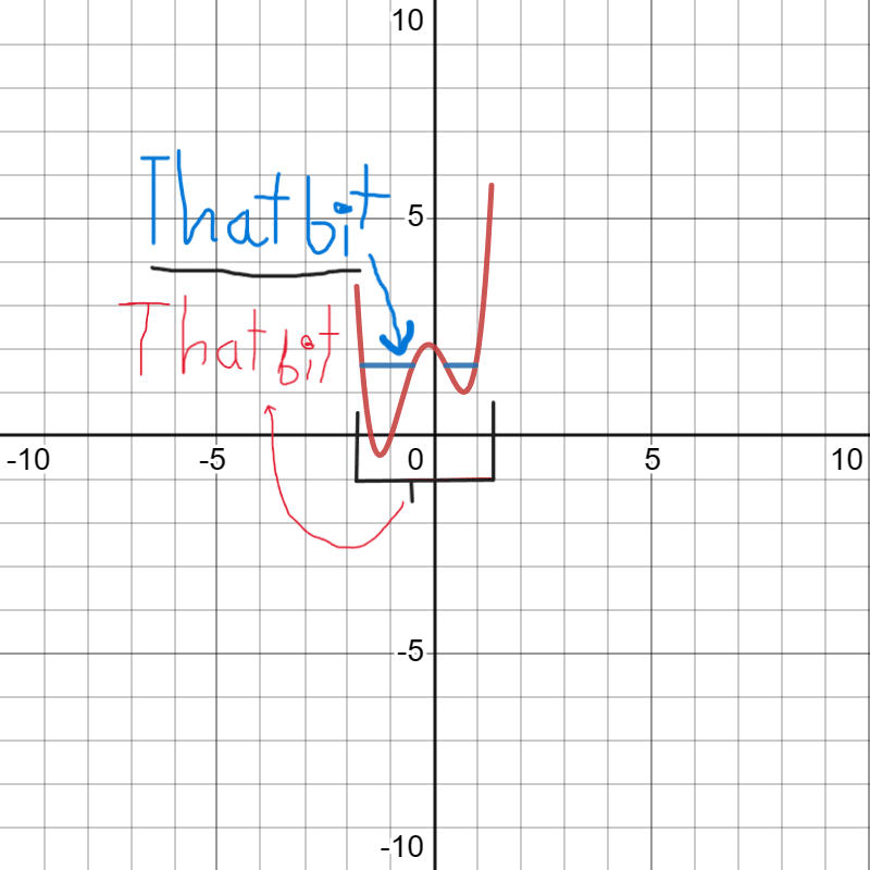
we randomly generate inputs for functions and use the largest value.

To get the expected value of this, we multiply each output by the probability that it's the highest using the function above, denoted as $f_i$, and then "add" all of those outputs to get the expected value.

Bringing it Together in $f_d$

Understanding the Mechanism of $f_d$:

$f_d$ calculates the expected value for each function  $f_1\left(x\right),f_2\left(x\right),and{f}_3\left(x\right)$​ individually and then multiplies them by how many times we "roll" them. ( $c_1,c_2,and{c}_3.$)

Component Analysis:

The full function is 

$f_d=\left({\int }_{a_1}^{b_1}\left(f_a{\left(f_1\left(x\right)\right)}^{\left(\frac{c_1-1+|c_1-1|}{2}\right)}{f}_b{\left(f_1\left(x\right)\right)}^{c_2}{f}_c{\left(f_1\left(x\right)\right)}^{c_3}{f}_1\left(x\right)\right)dx\right)c_1+\left({\int }_{a_2}^{b_2}\left(f_a{\left(f_2\left(x\right)\right)}^{c_1}{f}_b{\left(f_2\left(x\right)\right)}^{\left(\frac{c_2-1+|c_2-1|}{2}\right)}{f}_c{\left(f_2\left(x\right)\right)}^{c_3}{f}_2\left(x\right)\right)dx\right)c_2+\left({\int }_{a_3}^{b_3}\left(f_a{\left(f_3\left(x\right)\right)}^{\left(c_1\right)}{f}_b{\left(f_3\left(x\right)\right)}^{c_2}{f}_c{\left(f_3\left(x\right)\right)}^{\left(\frac{c_3-1+|c_3-1|}{2}\right)}{f}_3\left(x\right)\right)dx\right)c_3$

Let's focus on the first term:

$\left({\int }_{a_1}^{b_1}\left(f_a{\left(f_1\left(x\right)\right)}^{\left(\frac{c_1-1+|c_1-1|}{2}\right)}{f}_b{\left(f_1\left(x\right)\right)}^{c_2}{f}_c{\left(f_1\left(x\right)\right)}^{c_3}{f}_1\left(x\right)\right)dx\right)c_1$

This integral gives the expected value of $f_1\left(x\right)$ weighted by the probability that $f_1\left(x\right)$ has the highest output among the three functions for all valid inputs x.

Role of the Exponents: 

The exponents in the functions $f_a,f_b,and{f}_c$ serve a crucial role. Given that each of these functions essentially returns a probability, raising them to their respective exponents is the equivalent of multiplying the probabilities.

• $f_a{\left(f_1\left(x\right)\right)}^{\left(\frac{c_1-1+|c_1-1|}{2}\right)}$: Represents the probability that $f_1\left(x\right)$ is more than the value of $f_1\left(x_a\right)$, $c_1-1$ times. ($c_1$ is the number of times we "roll" an input for the function $f_1\left(x\right)$). The reason for the -1 is because we don't need to calculate the chances of $f_1\left(x\right)$ being higher than $f_1\left(x\right).$ The reason for the $\frac{+|c_1-1|}{2}$is because it outputs $c_1-1$ for all values where $c_1$ is more than or equal to $1$, and $0$ for all values less than 1. We do this because we don't want to get a negative exponent, as this may result in dividing by $0$, which is undefined.
• $f_b{\left(f_1\left(x\right)\right)}^{c_2}$ and $f_c{\left(f_1\left(x\right)\right)}^{c_3}$​ Represent the probabilities that $f_1\left(x\right)$ surpasses $f_2\left(x_b\right)$ and $f_3\left(x_c\right)$ respectively, the necessary number of times.

Enhancing your understanding

Probability of Being the Highest: 

By multiplying these terms, we calculate the joint probability that $f_1\left(x\right)$ is the highest output among the three functions a specific number of times as denoted by the coefficients, the same as you would if$f_2\left(x\right)$ were the same as a hypothetical $f_4\left(x\right)$, $f_5\left(x\right)$, ...^[1]

Weighting by the Function Value: 

Finally, we multiply this probability by the function's value $f_1\left(x\right)$ to weigh it by the actual outcome of the function, the same way you would always multiply probability by value.

Summing Over the Domain: 

By integrating over the domain of $f_1\left(x\right)$, we capture the aggregated effect across all possible inputs.

Applying the Coefficients $c_i$:

After obtaining the expected contribution of each function, we multiply each result by their respective coefficient $c_1$, $c_2$​, or $c_3$. These coefficients account for the number of times we evaluate each respective function in our simulation. 

We can then use the same logic for $f_2$ and $f_3$.

If you have any questions, I suggest you ask Chat-GPT or me. If you have any suggestions as to how I can make this clearer, or a better way of finding the expected value of the best option, or any wording that could be done differently, tell me. (ONLY if you want). No pressure.

If there's anything incorrect, please tell me.

Congratulations! You made it to the end!

as a special reward, have another funny video. You deserve it.

1. ^{^}

   3 Functions is an arbitrary quantity. you can use as many as you want. (Here's how)