Disclaimer: this is not a project from Alliance to Feed the Earth in Disasters (ALLFED).

Summary

• I estimated the future benefits of mitigating food shocks caused by abrupt sunlight reduction scenarios (ASRSs). These are scenarios in which a catastrophe causes a significant reduction in the amount of sunlight reaching the Earth’s surface, such as a nuclear winter, volcanic winter, or impact winter.
• The future benefits of globally mitigating the food shocks caused by an ASRS, conditional on it happening, are in the table below^[1].
  • Relative to the future benefits suggested by the guesses of Denkenberger 2022 for the reduction in far future potential, my estimates for an ASRS of:
    • 5 Tg^[2] are 1.80 % as large as those for a 10 % agricultural shortfall^[3] in its survey model, and 8.10 times as large as those in Anders Sandberg’s model.
    • 150 Tg are 22.9 % as large as those for a full scale nuclear war in its survey model, and 76.7 % as large as those in Anders Sandberg’s model.
  • In other words, my estimates for the future benefits are:
    • For mild ASRSs, much smaller than those from the survey, and larger than those from Anders Sandberg.
    • For severe ASRSs, smaller than those from the survey, and similar to those from the survey and Anders Sandberg.

• The future benefits of locally mitigating the food shocks caused by ASRSs vary significantly by country. Those of the 1st country, i.e. the one whose local mitigation leads to the largest future benefits, are:
  • For 5 Tg, 7.70 and 135 times as high as those of the 10th and mean countries.
  • For 150 Tg, 3.66 and 19.0 times as high as those of the 10th and mean countries.
• I think one should target democratic countries with large real GDP significantly affected by ASRSs, or ones which could plausibly influence them.

• All results should be taken with a big grain of salt, as they rely on quite speculative assumptions.

Acknowledgements

Thanks to Anders Sandberg, Anonymous Person, ChatGPT, Christian Ruhl, João Cortes, Lili Xia, Nuño Sempere, and Zvi.

Introduction

In this episode of The 80,000 Hours Podcast, William MacAskill said that:

It’s quite plausible, actually, when we look to the very long-term future, that that’s [whether artificial general intelligence is developed in “liberal democracies” or “in some dictatorship or authoritarian state”] the biggest deal when it comes to a nuclear war: the impact of nuclear war and the distribution of values for the civilisation that returns from that, rather than on the chance of extinction.

The distribution of values after a nuclear war depends on how the food shocks caused by the ensuing nuclear winter are handled, among other factors (e.g. degree of infrastructure destruction). This analysis quantifies the future benefits of mitigating food shocks caused by ASRSs. These are scenarios in which a catastrophe causes a significant reduction in the amount of sunlight reaching the Earth’s surface, such as a nuclear winter, volcanic winter, or impact winter.

Quantifying the future benefits of mitigating food shocks is relevant to more accurately assess the cost-effectiveness of interventions which aim to mitigate them. Denkenberger 2022 estimated the cost-effectiveness of planning, and research and development (R&D) for resilient food solutions in terms of increasing the value of the future. However:

• The models of Denkenberger 2022 rely on directly guessing the relative variation in the value of the future due to “full scale nuclear war” and “10% agricultural shortfall”. In contrast, my approach explicitly looks into the changes in values which supposedly lead to a worse future, which I believe is more informative.
• I present results by country and as a function of the amount of soot ejected into the stratosphere, which is less vague than the above terms.

My approach can also inform which countries should be targeted to develop preparedness and response plans for ASRSs. It allows one to estimate the future benefits of locally mitigating the food shocks in any given country.

Methods

Model and definitions

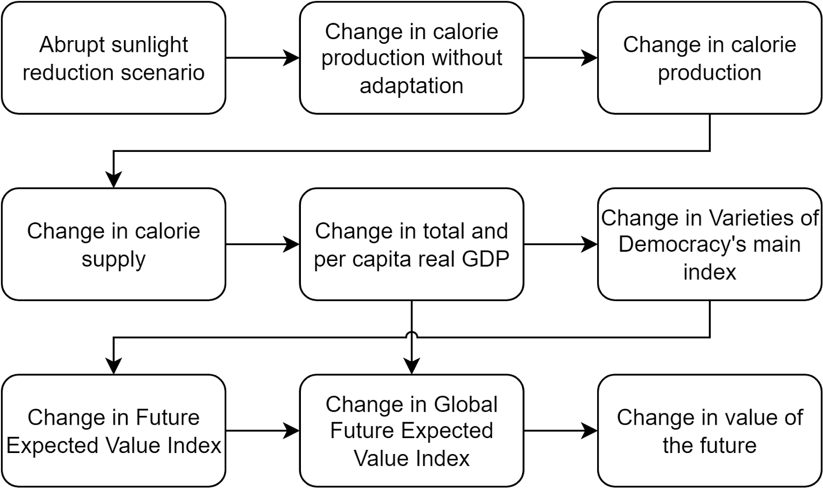
The diagram below illustrates how my model works. Note:

• I am only trying to quantify the future benefits of mitigating the food shocks caused by ASRSs. However, these have multiple other adverse consequences. For example, if caused by a nuclear war, ASRSs may involve loss of electricity and industry.
• The model is quite simplified, not including all pathways which will affect the value of the future. For instance, a change in calorie supply may well change factors besides total and per capita real GDP which influence Varieties of Democracy’s main index.

The Future Expected Value Index (FEVI) is the mean of 14 indices, rescaled to range from 0 to 1^[4], which look like decent proxies for future value (assessed for the baseline conditions in the last year for which I found data):

• Bertelsmann Transformation Index (2021), which “captures the extent of democratic features — political participation, rule of law, stable democratic institutions, political and social integration, and a capable state”.
• Economist Intelligence Unit's democracy index (2021), which “captures the extent to which citizens can choose their political leaders in free and fair elections, enjoy civil liberties, prefer democracy over other political systems, can and do participate in politics, and have a functioning government that acts on their behalf”.
• Environmental Performance Index (2022), which “provides a quantitative basis for comparing, analyzing, and understanding environmental performance”.
• Minus Global Peace Index (2022), which “is the world’s leading measure of global peacefulness”.
• Happy Planet Index (2019), which “is a measure of sustainable wellbeing, ranking countries by how efficiently they deliver long, happy lives using our limited environmental resources”.
• Human Development Index (2021), which “is a summary measure of achievements in three key dimensions of human development: A long and healthy life, access to knowledge and a decent standard of living”.
• Intergenerational Solidarity Index (2019), which “is a measure of how much different nations provide for the wellbeing of future generations”.
• Polity's democracy index (2018), which “combines information on the extent to which open, multi-party, and competitive elections choose a chief executive who faces comprehensive institutional constraints, and political participation is competitive”.
• Social Capital Index (2022), which “measures competitiveness of countries based on 189 measurable, quantitative indicators” “grouped into 6 sub-indexes: Natural Capital, Resource Efficiency & Intensity, Social Cohesion, Intellectual Capital, Economic Sustainability, and Governance Efficiency”.
• Social Progress Index (2022), which is “based on tiered levels of scoring that include measures in health, safety, education, technology, rights, and more”.
• Varieties of Democracy's main index (2021), which “denotes the best estimate of the extent to which political leaders are elected under comprehensive suffrage in free and fair elections, and freedoms of association and expression are guaranteed”.
• World Energy Council's (WEC’s) Trilemma score (2022), which “ranks countries on their ability to provide sustainable energy through 3 dimensions: Energy security, Energy equity (accessibility and affordability), Environmental sustainability”.
• World Happiness Report's (WHR’s) happiness score (2019 to 2021), whose “measure of SWB (Subjective Well-being) is from the Gallup World Poll (GWP)”.
• World Giving Index (2022), which aims to “establish a rounded measure of giving behaviour across the world” accounting for “helping a stranger”, “donating money”, and “volunteering time”.

I came up with 6 of these, and OpenAI’s ChatGPT suggested the other 8.

The Global Future Expected Value Index (GFEVI) is the FEVI across countries weighted by real gross domestic product (real GDP), which I suppose is a good proxy for (good or bad) influence in the value of the future.

I explain the model in the sections below, going from the start to the end of the causal chain. The calculations are in this Sheet (see tab “TOC”) and this Colab. I modelled all variables as independent distributions, and ran a Monte Carlo simulation to get the results^[5]. Additionally, I also estimated the key results from the table in the Summary using point estimates equal to the means of the distributions.

Calorie production without adaptation

I considered the ASRSs caused by nuclear wars of various levels of severity described in Table 1 of Xia 2022, which is reproduced below. The direct fatalities and people without food at the end of the 2nd year of the ASRS without adaptation increase linearly with the soot ejected into the stratosphere. The coefficients of determination of the respective linear regressions are 98.0 % and 96.7 % (see tab “Nuclear war fatalities”).

There is no consensus regarding the relationship between the amount of soot and nuclear weapon detonations^[6]. However, there seemingly is greater agreement on the climate and agricultural impacts given a certain amount of soot, and I present my results as a function of the amount of soot.

The relative variation in the calorie production without adaptation of major food crops^[7] and marine fish, from baseline to the 2nd year after the onset of the ASRS, is in Table S2 of Xia 2022 (see here). The values for the mean, and 5th and 95th percentile countries among the 167 analysed by Xia 2022 are below. The full data by country are in tab “Calorie production without adaptation”^[8].

I modelled the calorie production (for humans^[9]) without adaptation in the worst year of the ASRS as a fraction of its baseline value (CPWAf/CPWAi) as a rectified normal distribution^[10] with unrectified 5th and 95th percentiles equal to the minimum and maximum between (1 + RV)^2 and (1 - RV)*(1 + RV)^[11], where RV is the relative variation in calorie production without adaptation estimated in Xia 2022.

• The mean of the unrectified distribution is 1 + RV, i.e. it corresponds to the point estimate of Xia 2022.
• The distribution ensures the uncertainty, as measured by the distance between the unrectified 5th and 95th percentiles, is null when RV is -1 or 0, and maximum for RV = -0.5^[12], which makes sense.
• If Xia 2022 predicts no change (RV = 0) or total breakdown (RV = -1) in calorie production without adaptation, the distribution resumes to the point estimate CPWAf/CPWAi = 1 or CPWAf/CPWAi = 0.
• If Xia 2022 predicts a 50 % drop in calorie production without adaptation (RV = -0.5), I am supposing there would be a 5 % chance of the unrectified CPWAf/CPWAi being:
  • Lower than 25 %.
  • Higher than 75 %.

Calorie production

I determined the calorie production in the worst year of the ASRS as a fraction of its baseline value from CPf/CPi = (CPWAf/CPWAi)^E_CP_CPWA^[13], where:

• CPWAf/CPWAi is the calorie production without adaptation in the worst year of the ASRS as a fraction of its baseline value.
• E_CP_CPWA is the elasticity^[14] of calorie supply with respect to calorie production without adaptation.
  • This elasticity decreases with the level of preparedness and quality of the response to the ASRS^[15], and would be null for complete mitigation.
  • I set it to a normal distribution with 5th and 95th percentile equal to 0 and 1. So, for a decrease in calorie production without adaptation, I am assuming a chance of 5 % of calorie supply:
    • Increasing (E_CS_CPWA < 0).
    • Decreasing more in relative terms than calorie production without adaptation (E_CS_CPWA > 1).
  • For what is worth, ChatGPT’s best guesses for the 5th and 95th percentiles were -0.1 to 1, whose mean of 0.45 (= (-0.1 + 1)/2) is 10 % lower than mine of 0.5 (= (0 + 1)/2).
    • I only chatted with ChatGPT after defining my 5th and 95th percentiles.
    • You can see our chat here (ChatGPT’s guesses are in bold).

Calorie supply

I computed the calorie supply in the worst year of the ASRS as a fraction of its baseline value from CSf/CSi = (1 - CLWf/CPf)/(1 - CLWi/CPi)*CPf/CPi, where CLWf/CPf and CLWi/CPf are the calorie loss and waste^[16] in the supply chain as a fraction of the calorie production in the worst year of the ASRS and baseline conditions.

• I defined CLWf/CPf as the minimum between 1^[17] and a rectified normal distribution^[18] with unrectified 5th and 95th percentile equal to the minimum and maximum between (1 + RV)^2*CLWi/CPi and (1 - RV)*(1 + RV)*CLWi/CPi^[11].
  • The mean of the unrectified distribution is (1 + RV)*CLWi/CPi, i.e. it dictates the relative variation in calorie loss and waste equals that of the calorie production without adaptation predicted in Xia 2022. This is reasonable because less calorie availability will tend to result in less loss and waste.
  • The distribution ensures the uncertainty, as measured by the distance between the unrectified 5th and 95th percentiles, is null when RV is -1 or 0, and maximum for RV = -0.5^[19], which makes sense.
  • If Xia 2022 predicts no change (RV = 0) or total breakdown (RV = -1) in calorie production without adaptation, the distribution resumes to the point estimates CLWf/CPf = CLWi/CPi or CLWf/CPf = 0.
  • If Xia 2022 predicts a 50 % drop in calorie production without adaptation (RV = -0.5), I am supposing there would be a 5 % chance of the unrectified CPWAf/CPWAi being:
    • Lower than 25 % of CLWi/CPi.
    • Higher than 75 % of CLWi/CPi.
• I set CLWi/CPi to the fraction of 30 % applying to cereals mentioned here by the Food and Agriculture Organisation (FAO). This parameter would ideally be defined by country.

I thought about explicitly estimating for each country the elasticity of calorie supply with respect to calorie production^[20], but data on this is not readily available, so I opted to follow the approach described above for simplicity.

Real GDP

For the baseline conditions, I used the total and per capita real GDP and population of each country in 2021, which I took from these, these and these data from The World Bank.

For the worst year of the ASRS, I set the real GDP per capita of each country as a fraction of its baseline value to the minimum between 1 and RGDPC(CSf)/RGDPC(CSi), where:

• The real GDP per capita (RGDPC) is predicted with a linear regression of the daily calorie supply per capita on the reciprocal of the logarithm of real GDP per capita, fit to the available data of each of the 145 countries I analysed from 1960 to 2021.
  • The 145 countries are the ones for which there is data on Varieties of Democracy’s main index^[21], which I use to estimate FEVI (see next section).
  • 1960 and 2021 are the earliest and latest years encompassed by these data on real GDP per capita from The World Bank. For the daily calorie supply per capita, I used these data from Our World in Data (OWID).
• CSi and CSf are the initial and final daily calorie supply per capita, i.e. the ones in the baseline conditions and worst year of the ASRS.

As shown in the table below, the fit of the regression on the reciprocal of the logarithm of the real GDP per capita to data of the UK from 1789 to 2016, and of 145 countries from 1960 to 2021 is similar to other types of regression. Nonetheless, the one I selected leads to daily calorie supply per capita not increasing indefinitely with real GDP per capita^[22], which arguably makes sense. In any case, I assumed the real GDP per capita in the worst year of the ASRS could not exceed those in the baseline conditions^[23].

I presumed the population of each country as a fraction of its baseline value to be equal to the real GDP per capita of each country as a fraction of its baseline value (Pf/Pi = RGDPCf/RGDPCi). Consequently, I got the real GDP of each country as a fraction of its baseline value from RGDPf/RGDPi = (RGDPCf/RGDPCi)^2.

Note on real GDP per capita and cereal production

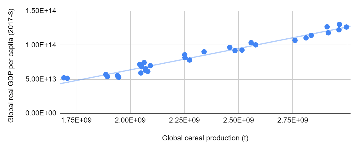
A unitary elasticity of real GDP per capita with respect to calorie production could naively be inferred from historical data. As is represented below, real GDP per capita increased linearly with global cereal production between 1990 and 2020 (coefficient of determination of 95.9 %; see tab “Global cereal production and real GDP”).

However, the aforementioned relationships are not necessarily causal:

• They are arguably explained by population growth causing real GDP per capita as well as cereal production to increase. In addition, higher real GDP per capita usually leads to higher consumption of animals (see this graph from OWID), which requires a greater calorie production.
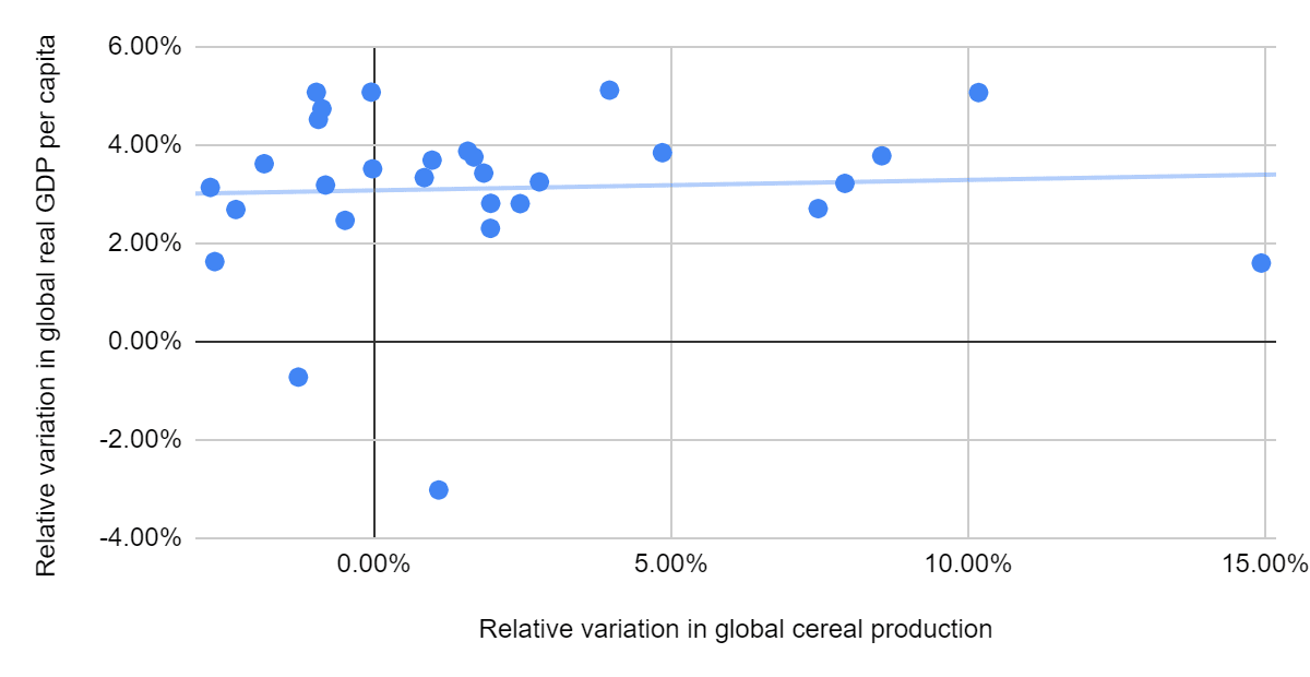
• The relative variation in real GDP per capita and relative variation in cereal production are only very weakly correlated (coefficient of determination of 0.421 %; see tab “Global cereal production and real GDP”), as is illustrated below. This suggests a low elasticity of real GDP per capita on calorie production.

For these reasons, I did not assume real GDP per capita to be directly proportional to the calorie production.

Varieties of Democracy’s main index

For each country, I computed Varieties of Democracy's main index (VoDMI) in the worst year of the ASRS as a fraction of its baseline value from VoDMI(RGDPCf)/VoDMI(RGDPCi), where:

• VoDMI is predicted with a logistic regression of it on the logarithm of real GDP per capita, fit to the available data of each country from 1960 to 2021^[26].
• RGDPCi and RGDPCf are the real GDP per capita in the baseline conditions and worst year of the ASRS. Further details are in the previous section.

This method is quite rough, but less resources per person (i.e. lower real GDP per capita) arguably lead to worse values. I used a logistic regression to predict VoDMI in the worst year of the ASRS because it corresponds to a S-curve with VoDMI tending to 0 and 1 (the minimum and maximum possible values) as the real GDP per capita tends to 0 and infinity. This valid asymptotic behaviour is good given the possibility of extreme variations of the real GDP per capita following ASRSs.

Sandberg 2021 argues “the future fit [of S-curves] tends to be poor unless the data covers the entire range from before to after the inflection point”. I do not think this is a major issue for my dataset. The mean weighted by 2021 real GDP of the number of data points per country with VoDMI lower and higher than 0.5 is 25.1 and 33.1^[27], so it looks like I have a good balance of points before and after the inflection point.

As shown in the table below, the fit of the logistic regression to data of the UK from 1789 to 2016, and of 145 countries from 1960 to 2021^[28] is similar to other types of regression^[29]. Nevertheless, I suspect the logistic regression will be a better predictor for large shocks for the reasons described just above.

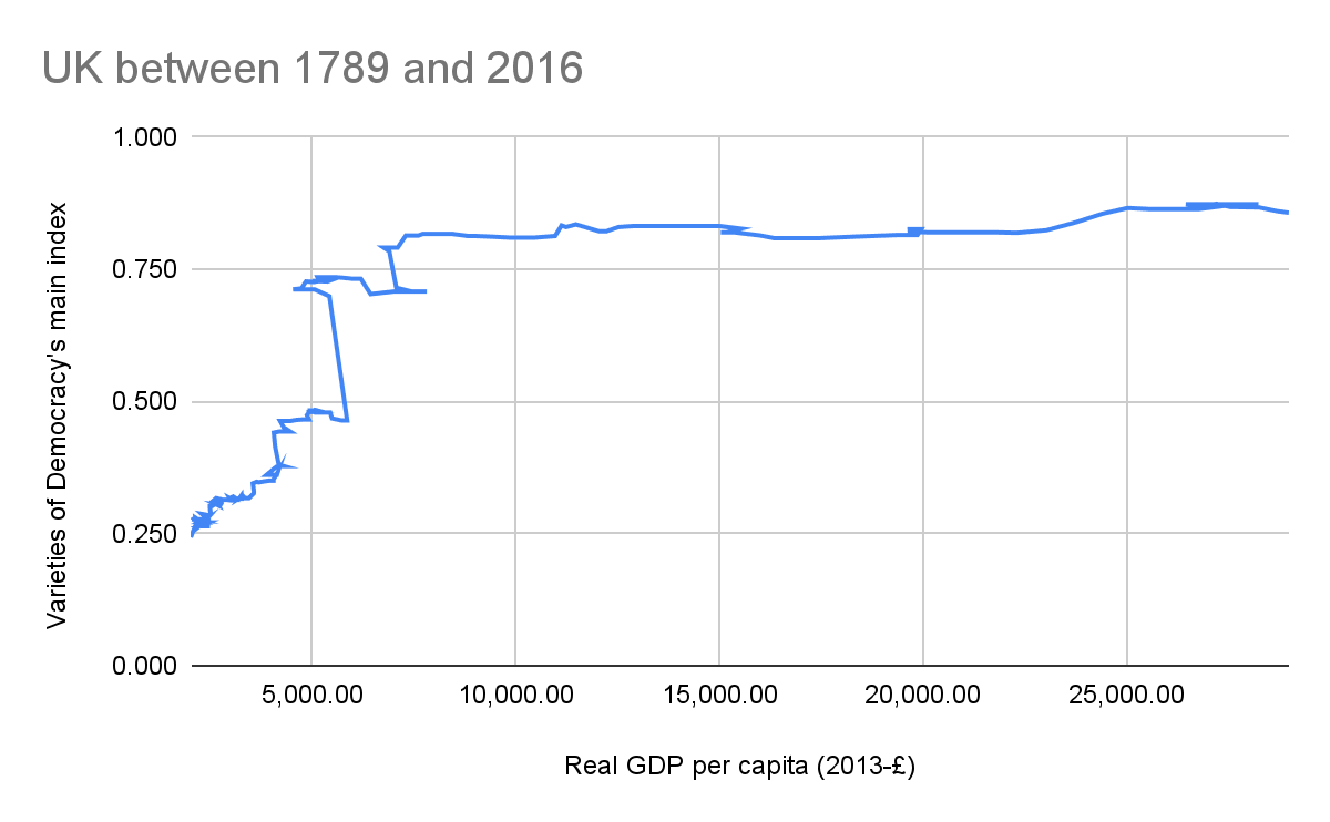
In any case, the figure below with data from the UK for 1789 to 2016 shows the logistic regression does not tell the whole story. Notably:

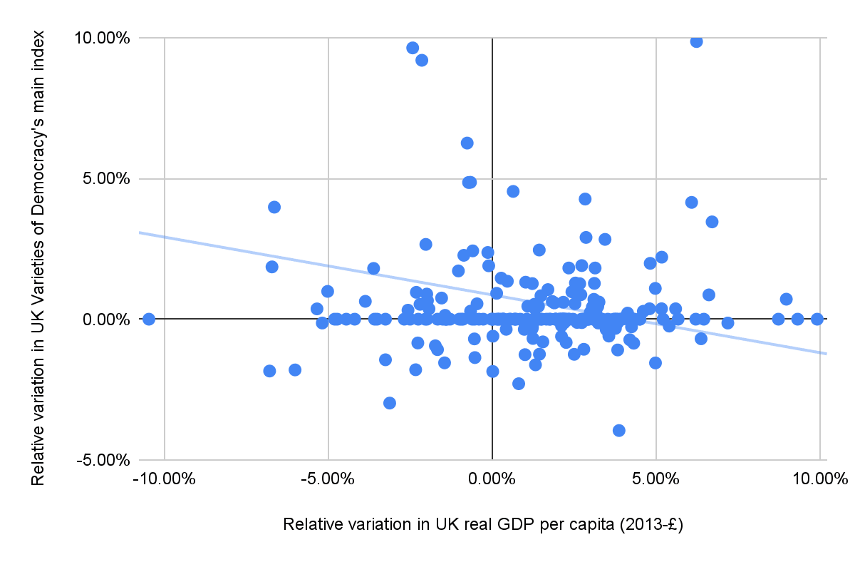
• From 1918 to 1919 (just after the end of World War I), real GDP per capita decreased 7.44 %, but VoDMI increased 50.6 % from 0.464 to 0.699.
• From 1920 to 1921, real GDP per capita decreased 10.5 %, but VoDMI remained constant.
• There were 4 transitions for which the real GDP increased significantly (8.73 % to 9.91 %), but VoDMI remained constant or barely increased (0.711 %).

In addition, as can be seen in the figure below^[31], the correlation between the relative variation in real GDP per capita and relative variation in VoDMI is negative, although it is pretty weak (coefficient of determination of 2.98 %).

Moreover, the logistic regression to estimate FEVI relied on the shorter period from 1960 to 2021, for which the fit is worse in agreement with the last row of the table above (51.6 % < 86.5 %).

Future Expected Value Index

For each country, I estimated FEVI in the worst year of the ASRS as a fraction of its baseline value from FEVI(VoDMIf)/FEVI(VoDMIi), where:

• FEVI is predicted with a linear regression on VoDMI, fit to the available data of 156 countries^[32] in the baseline conditions (see tab “Predicted FEVI”). The respective coefficient of determination is 79.9 %.
• VoDMIi and VoDMIf are the VoDMI in the baseline conditions and worst year of the ASRS (see previous section).

I did not directly estimate FEVI with a regression on the real GDP per capita due to:

• 12 of the 14 indices from which FEVI is calculated being quite recent.
  • Data for Polity’s democracy index and VoDMI goes back to 1776 and 1789, but only as early as 1990 for the others (see tab “Indices time frame”).
  • Data for the real GDP per capita is available from 1960, so there would be 30 (= 1990 - 1960) fewer years of such data for the other indices.
  • In turn, that would lead to significantly less data points before the inflection point of the logistic curve, and therefore poorer predictions (see Sandberg 2021).
• As illustrated in the table below, strong correlation for the baseline conditions between FEVI and VoDMI, for which data by country is readily provided by OWID here.

The 4 indices which correlate more strongly with FEVI for the baseline conditions are the Economist Intelligence Unit's democracy index (0.929), Social Progress Index (0.905), Rescaled Bertelsmann Transformation Index (0.895), and VoDMI^[33] (0.894). I relied on this to estimate FEVI in the worst year of the ASRS because the others are available for much shorter periods (in comparison to 1789 to 2021 for VoDMI):

• Economist Intelligence Unit's democracy index, 2006 to 2021.
• Social Progress Index, 2014 to 2022.
• Bertelsmann Transformation Index, 2005 to 2021.

The 2 indices which correlate more weakly with FEVI are the Happy Planet Index (0.373), and World Giving Index (0.232). Additional correlation coefficients are in tab “Correlations among real GDP, rescaled indices and FEVI”.

Value of the future

I estimated the value of the future after the ASRS as a fraction of its baseline value from VFf/VFi = (GFEVIf/GFEVIi)^(1 - RF), where:

• GFEVIi and GFEVIf are the GFEVI in the baseline conditions and worst year of the ASRS.
• RF is the recovery factor, which I set to a normal distribution with 25th and 75th percentiles equal to 0 and 1.
  • A value of 0 would imply a relative variation in the value of the future matching that of GFEVI (unitary elasticity). So I am assuming a 25 % chance the future would be worse than suggested by a given drop in GFEVI.
  • A value of 1 would imply no change in the value of the future (null elasticity), i.e. full recovery. So I am assuming a 25 % chance the future would be better for a drop in GFEVI.

1 - RF in the formula above is the elasticity of the value of the future with respect to GFEVI.

Finally, I determined the future benefits of mitigating a food shock caused by an ASRS as a fraction of the current value of the future from:

• If all countries completely eliminated the decrease in their real GDP and FEVI (global mitigation), (VFi - VFf)/VFi = 1 - (GFEVIf/GFEVIi)^(1 - RF).
• If a single country C completely eliminated the decrease in its real GDP and FEVI (local mitigation), (VFf*(C) - VFf)/VFi = (GFEVIf*(C)/GFEVIi)^(1 - RF) - (GFEVIf/GFEVIi)^(1 - RF), where GFEVIf*(C) is the GFEVI in the worst year of the ASRS if only country C completely eliminated the decrease in its real GDP and FEVI^[34].

These expressions indicate the scale of the risk of food shocks caused by ASRSs, but they are conditional on an ASRS happening. So they should be weighted by their probability to get a full picture of the risk. I plan to address this in a future post.

My formula for the future benefits of local mitigation calculates the counterfactual value, and therefore it does not account well for cooperation. Ideally, I should have used the Shapley value, as explained in this (great!) post from Nuño Sempere.

Parameters of the distributions

The distributions used in my Monte Carlo simulation are defined by many variables, but only 5 guessed constants (default values as mentioned in the previous sections):

• The 5th and 95th percentile elasticity of calorie production with respect to calorie production without adaptation (E_CP_CPWA_p5 = 0, and E_CP_CPWA_p95 = 1).
• Calorie loss and waste in the supply chain as a fraction of the calorie production in the baseline conditions (CLWi_CPi = 0.3).
• 25th and 75th percentile recovery factor (RF_p25 = 0, and RF_p75 = 1).

Feel free to make copies of the Sheet and Colab to use your own guesses (search for “Inputs” in the code). Copying the Sheet is needed because the Colab extracts data from there, and the copies must be in the same folder (unless you change the code).

Results

The results are in the tables below. The full results by country are in the Sheet (see tab “TOC”). For context, I also estimated the future benefits of mitigating food shocks caused by ASRSs based on the guesses of Denkenberger 2022.

Daily calorie supply per capita

Real GDP per capita and population

Real GDP

Varieties of Democracy’s main index

Future Expected Value Index

Global Future Expected Value Index

Future benefits of mitigating food shocks caused by ASRSs

Global mitigation

My results using a Monte Carlo simulation

My results using point estimates

Denkenberger 2022

Local mitigation

5 Tg

27 Tg

150 Tg

Discussion

Future benefits of mitigating food shocks caused by ASRSs

Global mitigation

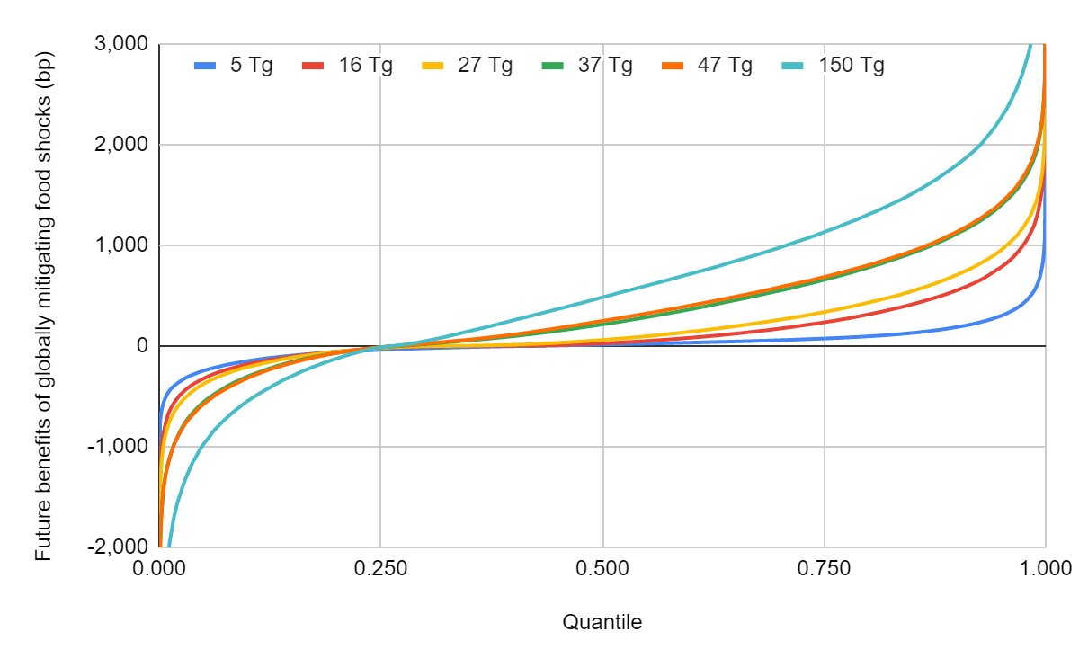
According to my results, the future benefits of globally mitigating food shocks caused by ASRSs as a fraction of the current value of the future are:

• For 5 Tg, 0.216 % (-2.44 % to 3.01 %, 5th to 95th percentile).
• For 27 Tg, 1.67 % (-3.75 % to 9.54 %).
• For 150 Tg, 5.54 % (-9.74 % to 22.7 %).

In addition, I estimate the probability of global mitigation being harmful decreases from 41.2 % for 5 Tg to 26.2 % for 150 Tg. This suggests even seemingly benign interventions to increase food security may prove harmful to the future. However, the heavy right of future benefits arguably makes their expectation robustly positive.

Relative to the future benefits suggested by the guesses of Denkenberger 2022 for the reduction in far future potential, my estimates for an ASRS of:

• 5 Tg are 1.80 % as large as those for a 10 % agricultural shortfall^[3] in its survey model (= 0.216/12.0), and 8.10 times as large as those in Anders Sandberg’s model (= 0.216/0.0266).

• 150 Tg are 22.9 % as large as those for a full scale nuclear war in its survey model (= 5.54/24.2), and 76.7 % as large as those in Anders Sandberg’s model (= 5.54/7.23).

In other words, my estimates for the future benefits are:

• For mild ASRSs, much smaller than those from the survey, and larger than those from Anders Sandberg.
• For severe ASRSs, smaller than those from the survey, and similar to those from the survey and Anders Sandberg.

Additionally, my results predict an ASRS of:

• 27 Tg to be 7.75 (= 1.67/0.216) times as bad as one of 5 Tg. In comparison, Xia 2022 estimates, without adaptation (see table here):
  • 3.59 (= 97/27) times as many direct fatalities.
  • 5.59 (= 1.426/0.255) times as many people without food at the end of the 2nd year.
• 150 Tg to be 3.32 (= 5.54/1.67) times as bad as one of 27 Tg. In comparison, Xia 2022 estimates, without adaptation (see table here):
  • 3.71 (= 360/97) times as many direct fatalities.
  • 3.75 (= 5.341/1.426) times as many people without food at the end of the 2nd year.

Finally, I am happy the results I got using point estimates (setting all distributions to their means) closely match the ones from the Monte Carlo simulation. The relative error of the point estimates ranges from -42.2 % for 5 Tg to 79.5 % for 150 Tg. These errors are not negligible. Moreover, one should be careful to set point estimates to means, which can be quite different from the medians or modes in heavy-tailed distributions. Anyways, even if the Monte Carlo simulation did not output significantly different expectations, it would still be useful to obtain a range of plausible results in a principled way (5th and 95th percentiles).

Local mitigation

The future benefits of local mitigation vary significantly by country. Those of the 1st country, i.e. the one whose local mitigation leads to the largest future benefits, are:

• For 5 Tg, 7.70 (= 38.2/4.96) and 135 (= 38.2/0.284) times as high as those of the 10th and mean countries.
• For 27 Tg, 12.1 (= 214/17.7) and 60.0 (= 214/3.57) times as high as those of the 10th and mean countries.
• For 150 Tg, 3.66 (= 858/234) and 19.0 (= 858/45.3) times as high as those of the 10th and mean countries.

Democratic countries with large real GDP significantly affected by ASRSs top the rankings of future benefits. Canada, Germany, Japan, and the United States are in the top 3, which is not surprising. Countries which are more democratic have higher FEVI^[38], and ones with larger real GDP have a greater influence in the value of the future (via having a greater weight in GFEVI).

For similar reasons, antidemocratic countries with large real GDP have the lowest ranking. China, Egypt, India, Iran, and Russia are in the bottom 3, being the ones for which local mitigation of food shocks is the most harmful to the future. There is a tension here:

• On the one hand, the worse antidemocratic countries come out of the ASRS, the less influence they will have over the future, and so the more democratic and better it will be.
• However, antidemocratic countries coming out of the ASRS worse entails greater suffering for the people living there.

To be blunt for the sake of transparency, in this model, the future would improve if the real GDP of China, Egypt, India, Iran, and Russia dropped to 0, as long as that did not significantly affect the level of democracy and real GDP of democratic countries. However, null real GDP would imply widespread starvation, which is obviously pretty bad! I am confused about this, because I also believe worse values are associated with a worse future. For example, they arguably lead to higher chances of global totalitarianism or great power war.

Additionally, my country rankings neglect important considerations. For instance:

• R&D on resilient foods conducted in one country may be leveraged by other countries.
• One country increasing its reliance against food shocks caused by ASRSs may motivate other countries to increase theirs.
• The cost (difficulty) of achieving my estimated future benefits will vary across countries.

All of these influence prioritisation among countries, so my rankings only offer a starting point. I think one should target democratic countries with large real GDP significantly affected by ASRSs, or ones which could plausibly influence them.

Metrics weighted by real GDP can be counterintuitive

My results apparently (but arguably not actually) underestimate the severity of the worst ASRSs. On face value, an ASRS of 150 Tg may seem more than 3.32 times as bad as one of 27 Tg, given this is 7.75 times as bad as one of 5 Tg. Moreover, the relative reduction in the value of the future increases linearly with the amount of soot (see 2nd table here).

I think the apparent underestimation of the severity of the worst ASRSs is explained by GFEVI being a mean weighted by real GDP. This may lead to counterintuitive conclusions if the real GDP in the worst year of the ASRS is concentrated in countries with socioeconomic indices much better than the current (real GDP weighted) average. This is possible:

• Xia 2022 estimates Australia’s calorie production without adaptation would increase 24.2 % relative to baseline for the ASRS of 150 Tg (see Table S2 here).
• As an extreme case, judging from this article by Steve Brusatte, the impact winter which played a role in the extinction of the dinosaurs contributed to the emergence of mammals. In turn, the shift in influence over the future towards mammals ultimately led to the rise of humans, who arguably have better values than dinosaurs.

Speculative assumptions

This analysis is quite shallow, and relies on somewhat speculative assumptions. By descending order of importance (to me):

• It is super unclear whether the structure of my model (see diagram here) meaningfully captures the dynamics which might lead to a worse future. In particular, it is quite high level, and does not explicitly model the possible infrastructure destruction due to the event which caused the ASRS, possibility of losing order due to civil or interstate wars, and collapse of governance.
• I guessed the recovery factor describing the elasticity of the value of the future with respect to GFEVI.
• I did not explicitly account for interactions between countries. Relatedly, I calculated the future benefits of local mitigation from the counterfactual value, instead of the Shapley value, which is better (see this post from Nuño Sempere).
• I guessed the parameters of the distributions describing the relationship between calorie production without adaptation and calorie supply.
• The worst year of the ASRS being the reference endpoint to calculate the future benefits (based on GFEVI) is a little arbitrary. Ideally, I would account for the whole duration of the ASRS.
• I modelled the relationships between calorie supply and real GDP per capita, and this and VoDMI based on historical data, from which causation cannot be robustly inferred.
• Such historical data may well provide a poor basis to predict what would happen in ASRSs, as it does not contain information about large food shocks. Between 1990 and 2020, the largest decrease in global cereal production was only 2.76 %^[39] (from 1994 to 1995).

That being said, explicit modelling increases reasoning transparency, and therefore enables criticism to be more constructive. So I believe it is better than relying solely on guesses.

Next steps

As next steps, it would be valuable to:

• Determine the probability distribution of the ASRS severity by year, which is arguably driven by the risk of nuclear war. I have a very early draft for this here.
• Do an analysis combining the one of this post with that suggested just above. This can include a sensitivity analysis to figure out which parameters drive the results, thus informing eventual further research.
• Leverage the findings about the risk of ASRS to more accurately assess and improve the cost-effectiveness of interventions which aim to mitigate it.

1. ^{^}

    The future can be quite valuable. For example, Nick Bostrom estimates here 10^38 human lives per century.

2. ^{^}

    1 Tg corresponds to 1 Mt.

3. ^{^}

    Xia 2022 predicts a shortfall of 7.0 % for 5 Tg without adaptation (see last row of Table S2).

^{^}

 Rescaling the indices is not only useful to define FEVI, but also to make comparisons between different indices.

^{^}

 For 100 k random samples per variable, the Colab takes me 50 min to run, but only 3 min without computing the future benefits of local mitigation (changing “local_mitigation = True” to “local_mitigation = False” at the top).

^{^}

 This relationship is discussed in Toon 2008, Mills 2014, Denkenberger 2018, Reisner 2018, Toon 2019, Wagman 2020, and Hess 2021.

^{^}

 Maize, rice, soybean, and spring wheat.

^{^}

 I replaced the occurrences of “-100.0 %” by -99.975 % (= -(100 % + 99.95 %)/2). The 167 nations studied by Xia 2022 encompass the 145 countries for which there is data on VoDMI.

^{^}

 Excluding calories produced for animal feed or biofuels.

^{^}

 Maximum between 0 and a normal distribution, which makes sense given calorie production cannot be negative.

^{^}

 The formulas swap when the sign of RV changes.

^{^}

 The distance between the unrectified 5th and 95th percentiles is -2*RV*(1 + RV), which is a parabola with zeros -1 and 0, and maximum 0.5 for RV = -0.5.

^{^}

 Except for the samples with null CPWAf/CPWAi, in which case I set CPf/CPi to 0 (the other formula would produce infinities for samples with null CPWAf/CPWAi, and negative E_CP_CPWA).

^{^}

 The concept of elasticity is often used in economics to model how the change in one variable affects the change of another variable (see this page from Wikipedia).

^{^}

 For example, the extent to which calories used for animal feed and biofuels are directed toward human consumption.

^{^}

 According to this article from Maryam Rezaei and Bin Liu:

- “Food loss is mainly caused by the malfunctioning of the food production and supply system or its institutional and policy framework. This could be due to managerial and technical limitations, such as a lack of proper storage facilities, cold chain, proper food handling practices, infrastructure, packaging, or efficient marketing systems”.

- “Food waste refers to the removal from the food supply chain of food which is still fit for human consumption. This is done either by choice or after the food is spoiled or expired due to poor stock management or neglect”.

^{^}

 The calorie loss and waste cannot exceed the calorie production.

^{^}

 Maximum between 0 and a normal distribution, which makes sense given calorie loss and waste cannot be negative.

^{^}

 The distance between the unrectified 5th and 95th percentiles is -2*RV*(1 + RV)*CLWi/CPi, which is a parabola with zeros -1 and 0, and maximum 0.5*CLWi/CPi for RV = -0.5.

^{^}

 The elasticity of calorie supply with respect to calorie production is the slope of a linear regression of the logarithm of calorie supply on the logarithm of calorie production. Data on calorie production could be derived from FAOSTAT’s data about the quantity of food produced in terms of mass, and caloric density tables.

^{^}

 See cells for which there is data in column T of tab “Indices for baseline conditions”.

^{^}

 The regression on the reciprocal of the real GDP per capita also has this property, but it is more common to deal with the logarithm of real GDP per capita.

^{^}

 This has the technical advantage of preventing overflow errors in the estimation of the real GDP per capita in the worst year of the ASRS.

^{^}

 Calculated in tabs “Calorie supply and real GDP per capita” and “UK calorie supply and real GDP per capita”.

^{^}

 1990 and 2020 are the earliest and latest year for which The World Bank has data about the real GDP and cereal production. I used these data from The World Bank for the cereal production.

^{^}

 For each country, I only considered the years with data for both the real GDP per capita and VoDMI. The former was the limiting factor for all countries except Kazakhstan and Montenegro, which had data in 1990 and 1997 for the real GDP per capita, but not VoDMI. To prevent this from being the sole limiting factor, I estimated VoDMI for Kazakhstan in 1990, and Montenegro in 1997 via linear interpolation.

^{^}

 See O2:P2 of tab “V-Dem's main index and real GDP per capita”.

^{^}

 For the historical real GDP per capita, I relied on these data from OWID for the UK, and these from The World Bank for the 145 countries.

^{^}

 Except for that of the linear regression to data of the UK, as 61.9 % is materially lower than 86.6 %.

^{^}

 Calculated in tabs “V-Dem's main index and real GDP per capita” and “UK V-Dem's main index and real GDP per capita”.

^{^}

 The point respecting the relative variations from 1918 to 1919 is the only which is not visible.

^{^}

 The ones analysed by Xia 2022 with available data for the real GDP from The World Bank.

^{^}

 Rescaling does not change the correlations (see here).

^{^}

 For the cases in which calorie production increases, there is no decrease in real GDP nor FEVI to be eliminated, so GFEVIf*(C) = GFEVIf, and there are no future benefits.

^{^}

 Calculated with this Sheet, which is presented here.

^{^}

 According to David Denkenberger, the survey was conducted in 2018.

^{^}

 Calculated from the product of the means in the previous tables, since all distributions were assumed to be independent in Denkenberger 2022.

^{^}

 There is a correlation in the baseline conditions between VoDMI and FEVI of 0.894 (see last table here).

^{^}

 See tab “Global cereal production and real GDP”.

Show all footnotes