Disclaimer: I can’t be sure I didn’t make any errors here. If you spot any clear factual errors or mistakes in the code, feel free to message me.

Introduction:

In my last post, I gave an overview of the “optimizer’s curse”^[1] an important and underdiscussed phenomenon that where the ranking of causes by fallible estimators leads to a (sometimes dramatic) overestimate of the top cause. In that post, I used a toy model to demonstrate the curse in action for a simplified charity ranker, showing a sizeable effect, especially for very uncertain causes.

When using a model, it is always important to do a little intellectual exploring. We might want to ask: Does the curse still apply for distributions that aren’t normal? Does the curse still apply if estimators are biased towards pessimism? Can you mitigate or correct the curse by adopting a “portfolio” of effective charities?

In this post, I will take that toy model and play around with it to try to answer these questions and more. I aim to show how different assumptions and tweaks affect the results, and examine how robust the resulting effect is.

I want to caution that even with the added complexity explored in this post, I am still discussing a simplified model of reality. The goal here is to get a better intuition about how the curse works, what conditions should make us worried, and some ideas about how to correct for it. I would also encourage people to read the original paper, as well as this article and this article exploring the phenomenon.

I will break this article into 6 “experiments”, each exploring a different aspect of the curse. Feel free to skip any that seem boring to you.

There will be some technical details, but on the other hand there will also be a lot of pretty graphs. The code I wrote for this post is available here: it is hopefully somewhat improved compared to the last post.

Refresher on basic model:

Feel free to skip this section if you read my last post.

The base model we are using is described in detail in my previous article. Essentially, we simulate the ranking of charities by supposing that there are two distributions, one of the “actual effectiveness” of charities, and one of the error we make when we estimate charities. When we pick out a new charity to evaluate, we are taking the actual effectiveness, and adding on the error to get our estimated effectiveness.

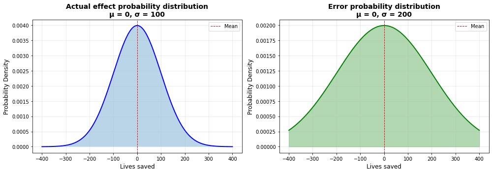
For the sake of easily seeing the curse, we will use the “speculative” class of charities from the last post as the base model. This is supposing we are grabbing from distributions where the range of errors is twice as high as the range of the actual effectiveness.This is very roughly modelled after the “deworm the world” uncertainty range shown in this post. All “lives saved” numbers are taken to be “per million dollars”, which was chosen to very roughly align the top charity effectiveness with Givewell’s top charity estimate of ~250 lives saved per million dollars.^[2] For information on how Givewell corrects for the curse in their estimates, see the section on the topic in my last post.

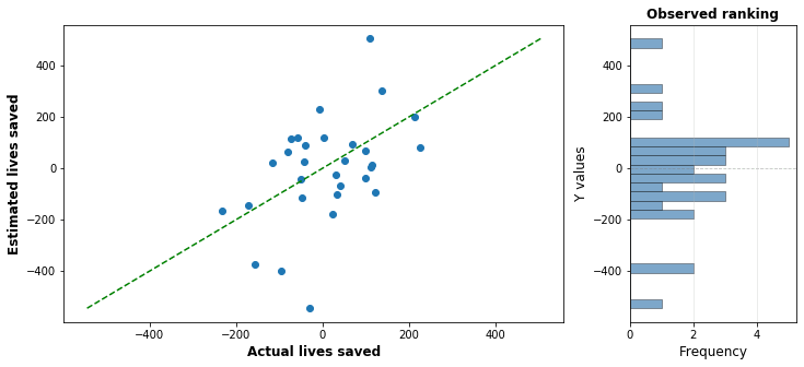
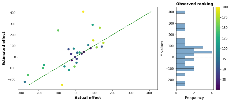
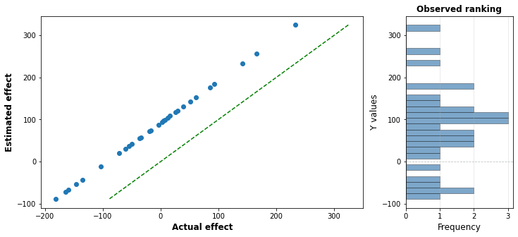
Increasing the number of charities we pick increases the chance we pick out a high performing charity: but it also increases the chance that we will pick a large positive error that causes a charity to be wrongly bumped up in the rankings. The following graph shows one simulated run with 30 charities, with the actual effect graphed against the estimated effect: the distance above or below the green line indicates how much the charities effectiveness has been under or overestimated. The top charity in this run has an estimated effectiveness of around 400 lives saved per million dollars, when in reality it only saves 30 or so.

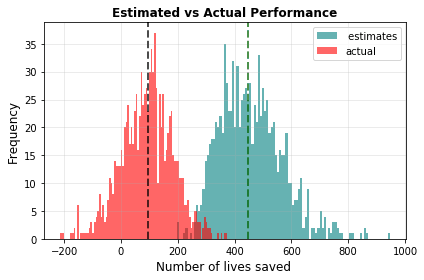
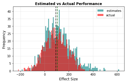
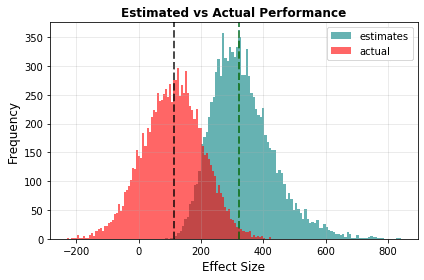
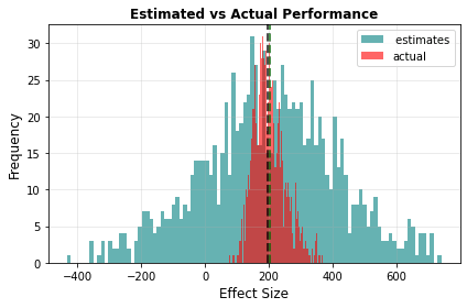
By graphing the performance of the top result over thousands of simulation runs, we can demonstrate the curse in action. In the graph below, the median of the estimates (in teal) is much higher than the median of the actual effectiveness (in red).

There is also an important effect where uncertain causes are unfairly favoured over certain ones, but I will revisit this in experiment 2.

Experiment 1: Biased error

In the original model, I assumed that the error made on each intervention estimate was symmetrical: that you were equally likely to overestimate and underestimate the error. How important is this assumption? If your estimates were biased to underestimate causes, would that counteract the effect?

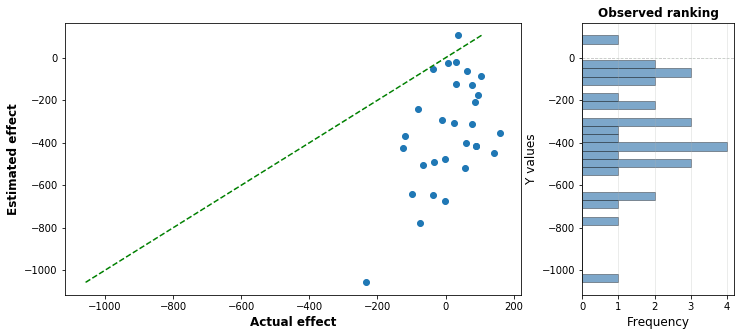
Well, I tried it out with the settings above, and found the error bias you’d need, with error standard deviation 200, to cancel out the effect of the optimizer’s curse. Feel free to guess how much it needs to be, I’ve shown one run of the estimation below:

The answer is around -350: that is, we underestimate every single charity by an average of 350 lives. Keep in mind that the best actual intervention is only around 200 lives. This is massively biased against each charity: you underestimate the true value of each charity roughly 95% of the time.

So in isolation, the estimates for each charity are horribly wrong. And yet, if we look at the performance of the top charity, we get a different story:

This horribly biased error ends up cancelling out the optimizer’s curse, and ensuring that the estimate of the top intervention is spot on. In retrospect, this is actually kinda obvious: with no bias the overestimate of the top charity is around 350 lives, so the bias has to counter this exactly.

To be clear, I’m not recommending that you try and be horribly pessimistic when evaluating charities. You can see the previous post for a much better way of compensating for the curse, where a weighted average of the calculated estimated and a prior estimate is used.

Conclusion:

Even if your evaluators are overly pessimistic, it might not be enough to counteract the curse: they have to either be very pessimistic, or they have to be pessimistic in the right way.

Experiment 2: The cost of uncertainty

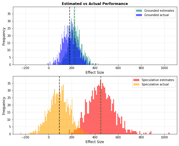
An interesting aspect of the optimizer’s curse is that as uncertainty grows, the estimated effectiveness of an intervention shoots up, but the actual effectiveness goes down. We can see this by comparing two interventions, a grounded intervention with a low error standard deviation (50), and a speculative one with a high error standard deviation (200): the following graph shows the performance of the top charity:

The actual effectiveness of the top grounded charity, in Blue, is about twice that of the top speculative charity. This occurs because each grounded estimate is more trustworthy than each speculative estimate, allowing the ranking of charities to be more accurate and to therefore give us a higher actual result.

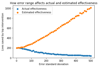
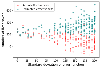
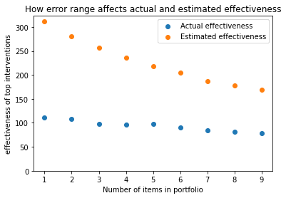
In the next graph, I have visualised how the actual and estimated effectiveness varies as you vary the uncertainty (error standard deviation). We graph the error standard deviation against the median actual and estimated effectiveness over a thousand runs. All other parameters are kept the same as the baseline model:

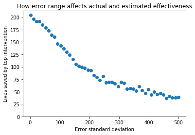
We can see the strong divergence between estimated and actual effectiveness as uncertainty increases. It’s hard to see the shape of the blue curve, so in the next graph, I will zoom in on specifically the actual effectiveness.

I think this is quite interesting, because it allows us to directly show how reducing uncertainty translates to lives saved. Consider the following riddle:

Imagine you live in Idealistan, a country where all the assumptions of our simplified model are correct. You are entrusted with 100 million dollars, which you want to direct as effectively as possible. You are picking between 30 possible interventions. You have the choice between doing the charity evaluation in-house, where you think the error standard deviation for each charity will be 200 lives per million, or hiring expensive outside contractors to do indepth research on each intervention that will bring the error standard deviation down to 50 lives per million. If you want to maximize lives saved, how much would you be willing to pay the contractors, if the alternative is donating the extra money to charity?

Feel free to take a guess or solve it yourself if you feel like it.

Under the above model, the top identified charity when error stdev is 200 will save 85 lives per million dollars, whereas the top identified charity when error stdev is 50 will save 181 lives per million dollars. So switching from one to the other will save 96 lives per million dollars. If we multiply this by the 100 million endowment, switching from one to the other will save 9600 lives.

To save that many lives with the top identified (200 stdev) charity would cost 53 million dollars.

Therefore, you should be willing to spend up to 53 million dollars, or 1.75 million dollars per intervention, to hire the contractors. That’s more than half the endowment!

Now, I’m not endorsing spending half your endowment on charity ranking in real life. I’m strictly talking about Idealistan here, for this particular case with this particular distribution of actual effectiveness I think it’s still a good illustration of just how powerful lowering uncertainty can be.

Conclusion:

The optimizer’s curse shows us a way in which uncertainty directly costs lives: more uncertain interventions show large growth in estimated effectiveness, while their actual effectiveness decreases. Under certain circumstances, actively working to reduce uncertainty can be highly cost effective.

Experiment 3: Continuous variation in uncertainty

In the original model, the uncertainty range for each intervention was the same for every intervention^[3]. In this experiment, I change this so that each intervention has a different error standard deviation. I could have made a complicated model, but I opted to just have each intervention in the run be sampled from a curve with different stdev, varying linearly from 1 to 200.

In the following graph, I show one run of this experiment, with the error standard deviation of each point coloured in, with darker points being less uncertain and lighter points being more uncertain:

You can clearly see that the lightly coloured dots are off by much larger amounts then the dark dots, and that the top apparent charities have a disproportionate number of uncertain charities.

Next, we see the optimizer’s curse in action: the actual lives saved has a median of 111, whereas the median estimated lives saved is 321, a 210 life overestimate:

In the following graph, I plotted a scatterplot of the top charities, graphing their error standard deviations against their estimated effectiveness (teal) and actual effectiveness (red).

You can see that the left side is more sparsely populated than the right, indicating that the selection process is highly biased towards picking high uncertainty interventions. You can also see the same divergence of effectiveness as we saw in the last experiment.

Conclusion:

Optimizer’s curse effects persist if each intervention has a different uncertainty level. Our experiments showed, as before, the way that the optimizer’s curse biases us toward uncertain causes.

Experiment 4: Changing shapes and skews

In our model so far we have made the assumption that both the actual effectiveness and error range are sampled from normal distributions. This is a common assumption to make, but it’s unlikely that either of these will perfectly follow a normal distribution in real life.

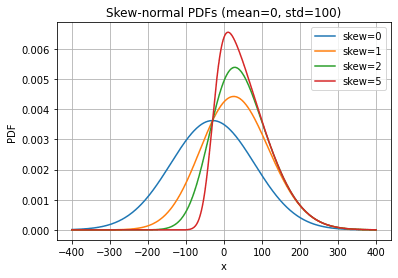
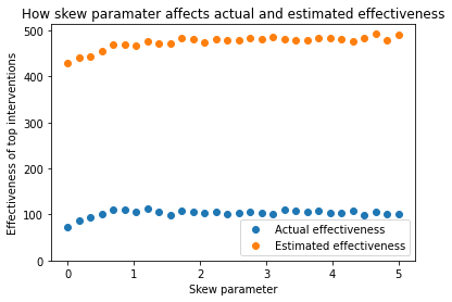
As one example, we might take issue with the assumption that charity intervention is perfectly symmetric. One could argue that the vast majority of charities are actually trying to make the world a better place, even if they don’t always succeed. I might decide to model the actual effectiveness therefore as a skew-normal distribution like the following:

The various curves here show the effect of varying the “skew parameter”. The red curve here seems to capture some intuition about charity effectiveness: Most charities are not very cost effective at saving lives, and most charities do not actively set out to harm people, although a reasonable chunk are net negative by accident.

This gives a concern: although the different skews do have different shapes, their shape at high values is virtually identical with skew 1 and above. This is an important thing to emphasize: the shape of the highest part of the curve is what matters the most.

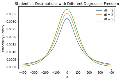
We can see this much more starkly if we switch from exploring skew to exploring “long-tailedness”. The following graph shows three distributions that look pretty similar:

These are students t test curves, with different “degrees of freedom” (DF) factors. An infinite DF value is just a regular normal curve. As DF approaches 1, it approaches a Cauchy curve: a curve with extremely long “tails”. In a long tailed distribution, most of the values are clustered together, but the outlying values are massively higher than regular ones.

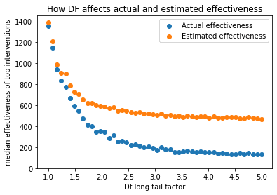
In the following graph, we can see the effect that this has on actual and estimated effectiveness:

So we can see that as DF decreases, corresponding to long-tailed charity distributions, the magnitude of the optimizer’s curse decreases, to the point where estimates match with actual effectiveness pretty well.

You could say the reason for this is that you are cranking up the gap between the top and the 2nd intervention to the point where standard errors can’t overcome it: a similar effect will happen if you crank up the standard deviation of the actual effectiveness curve.

Conclusion:

The shape of the distribution of actual effectiveness may affect the optimisers curse. A test with a skewnorm distribution found that right skewed distributions did not significantly affect the curse, but a test on long-tailed distributions found that very long-tailed distributions have reduced curse magnitude. Particular attention should be paid attention to the shape of the effectiveness curve at high positive values.

Experiment 5: Portfolio strategies

Most of the writing and modelling here has been focused on looking at the top charity on it’s own. This might give people the false reassurance that you don’t have to worry about the curse if you’ve spread your investments across a number of different top interventions, adopting a strategy where you have a portfolio of interventions.

This isn’t true. Sure, the top charity is the most affected by the curse, but the 2nd from the top is as well, as is the third, etc. If you average the top 3, you aren’t eliminating the curse, just lessening it’s impact.

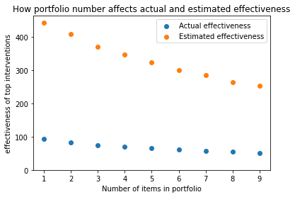
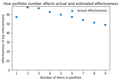
I wrote some code that looks at the effectiveness of a strategy where resources are divided evenly among the top n interventions In the following graph, I show how the size of a portfolio affects effectiveness for our standard case:

As portfolio size increases, the overestimate decreases, but there is still a substantial overestimate. And if you look at the actual effectiveness of your investment strategy, it goes down as the number of items goes up. If your goal is to maximise expected lives saved, even accounting for the optimizer’s curse the best strategy is still to just pick the top charity.

That’s not the end of the story though, because this was a model where all the interventions have equal uncertainty. In cases where interventions vary in uncertainty in unknown ways, I can make a case for portfolio tactics by stating that a portfolio of items is more likely to grab the low uncertainty interventions that are unfairly passed over despite being better on average than high uncertainty interventions.

I can show this by creating a model in which almost all of our charities have the same uncertainty, but there is one hidden charity that is actually 10 times as uncertain as the others. In this case, a portfolio strategy is an improvement

However, I tested the portfolio on our “variable standard devs” from experiment 3, and I still got decreased value from portfolio strategies:

We are still talking just about our toy model here, and there are other reasons to prefer a portfolio of charities: for example some impactful charities only have enough capacity to absorb certain amounts of funding.

Conclusion:

In a case where the uncertainties of interventions are similar to each other a portfolio strategy will lessen the magnitude of the optimisers curse, but at the cost of reducing the actual effectiveness of your investment strategy. I showed one example where if one charity is significantly more uncertain than others, the portfolio strategy will pay off if the portfolio is small. I think more investigation of portfolios might be warranted, but it seems clear they are not a silver bullet solution to the curse.

Experiment 6: Correlation:

One assumption of the simple model is that the errors in estimating each intervention are completely independent from each other. This is unlikely to be true. The estimations of many different charities may share assumptions, and an error in these assumptions will affect multiple estimates at once. For example, an error in the estimated malaria prevalence in Uganda will affect the estimated effectiveness of both a malaria vaccine charity and a malaria bednet charity, making their estimates incorrect in different ways.

Correlation can get pretty complicated, but I tried to find the simplest possible model that can demonstrate the effect. In this model, a “global” error is sampled from the error distribution, which is the same for each intervention, and then each intervention has it’s own “local” error sample. The final error is then taken as a weighted average of the “global” error and the “local” error, with a correlation factor F saying what fraction of the “global” error is taken.

I’ve drawn a crude diagram of an example calculation, but don’t worry too much if it’s confusing. It’s not meant to be an accurate representation of correlation in the real world, but a way to get across why correlation is important:

If our correlation factor F is 0, then we have independent errors and the result is the same as before.

If our correlation factor F is 1, then we have a situation where the estimate of every single intervention is off by the exact same amount. One run of this is shown below:

You can see that all points are the exact same vertical distance from the line of accuracy. Because of this correlation, there is no way for a lower effectiveness charity to “leapfrog” a higher one, so the order will be exactly right. As a result, there will be no optimizer’s curse in the result, although you might still be quite wrong in your estimates:

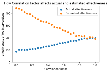
Full correlation like this seems quite unlikely to happen in practice. The following graph shows what happens in between zero and full correlation, as we change our correlation factor F:

We can see that as the correlation increases, the magnitude of the optimizer’s curse decreases, and the actual effectiveness of the top charity climbs as well.

I really could not tell you how much of an effect this has in real charity evaluations. In reality, not every cause would be super correlated, but some would be highly correlated: it’s easy to see how there could be correlations between different malaria vaccine programs, but there probably isn’t that much correlation between malaria vaccines and cash transfers. You’d need a more complex model to figure out the magnitude of this effect, but I think high correlation factor equivalents are unlikely.

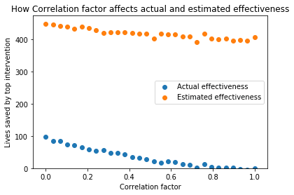
Before we leave, it’s worth noting that the sampling of the charities themselves could also be correlated: perhaps there is a Ugandan person on the staff who knows more charities in that country, so Ugandan charities are preferentially picked, which have higher effectiveness on average. This type of correlation would have the opposite effect to error correlation, making the optimizer’s curse worse. I ran the same procedure as above, but applying it to the actual effectiveness rather than the error, and got the following results:

This shows that as the results of the actual charity sampling become very correlated, the benefits of charity ranking drops to zero, which is what you’d expect, because the charity effectiveness end up being exactly the same.

Conclusion:

A simplistic demonstration shows that correlation of errors reduces the magnitude of the optimizer’s curse. As a result, the magnitude of the optimizer’s curse in reality will be less than our original model says, but it is tricky to model this for real applications. Correlation of the sampling of actual causes will have the opposite effect and make the curse worse.

Overall conclusion:

I covered six experiments:

In experiment 1, I looked at whether pessimistic bias in individual error estimates could cancel out the optimizer’s curse, and demonstrated that you would have to be unreasonably pessimistic to cancel it out.

In experiment 2, I looked at how uncertainty affects the actual effectiveness of top selected charities, and showed some model assumptions under which cutting uncertainty could directly result in saving extremely large amounts of lives.

In experiment 3, I looked at what happens if the uncertainty of every charity is different: this largely backs up the bias toward uncertain causes mentioned elsewhere.

In experiment 4, I looked at how the shape of the actual effectiveness distribution affects the results: a skew towards the right has very little effect, but an increase in long-tailedness can dramatically increase actual effectiveness and drastically reduce the magnitude of the optimizer’s curse.

In experiment 5, I looked at whether portfolio tactics defeated the optimizer’s curse, and generally found that at least in this model, they had some effect but did not actually lead to better actual results under most circumstances.

In experiment 6, I examined the effect of correlation, showing that if errors are not independent of each other, the magnitude of the optimizer’s curse decreases.

These experiments are by no means exhaustive: reality is always more complicated than simple models can capture. However, it looks to me like the effect is robust enough to changes in assumptions that we should expect to see it to some extent in a wide range of circumstances.

One area I did not explore was what happens when uncertainty gets really big: this will be the subject of a followup post.

These experiments were conducted in order to try and get a feel for how robust the optimizer’s curse effect is, and how much a few of our simple model assumptions affect it. My impression after doing all of this is that the effect is pretty robust, and that most charity rankings with roughly similar characteristics to the toy model will exhibit the optimizer’s curse unless it has been actively corrected against.

1. ^{^}

   I’ve switched to the American spelling of “optimizer” to be consistent with the original paper.

2. ^{^}

   Using their estimate of 3000-5500 to save a life, the range of lives saved by a million dollars is 180 to 330. If this error range was a 95% probability interval, then the estimated uncertainty SD is around 40 lives, similar to the “grounded” intervention from last post.

3. ^{^}

   Except when comparing grounded to speculative.