Johannes Ackva, Megan Phelan, Aishwarya Saxena & Luisa Sandkühler, November 2023
Context for Forum Readers:
This is the methodological component of our Giving Season Updates, originally published here and leaning heavily on our recent EAGx Virtual talk available here.
This post can be understood as an update to our post from May outlining our methodological vision.
We have also published a much briefer update on our 2023 highlights here.
Main text:
“What is impact maximizing in taking philanthropic action in climate and why do we believe this?”
In this piece, we are trying to answer how we think about answering this question (rather than the substantive answer itself, see below for our view on the latter), why we think this is a hard question and why we think we can and have made progress in answering this question.
It is a pretty fundamental piece, meant for people interested in getting an introduction to our methodology, our reasoning, and how we make claims about relative impact.
Before we dive in, here are a couple of pointers to other resources that address other related questions: Here we provide a quick summary of our view on 2023 highlights and on “time-stamped” developments, and here we collect all resources FP Climate and host the Climate Fund, the primary vehicle through which we put our research into action making a driving change in the world (you can contribute here, or – if you are a member – talk to your advisor or community manager). Here you can find our last big picture update on all things climate (we hope to update this in early 2024) and here and here you can listen to it.
Adapted from a talk, we also try to keep this piece conversational, light, and relatively informal.
Now, let’s dive in!
The Problem: Maximizing impact under high uncertainty
There are at least two ways of looking at why trying to answer the question “where should I give in climate to maximize my positive impact?” is a hard one and we briefly discuss both. As this is fundamentally an optimistic piece – things are hard but not impossible! – we then discuss how we believe we can still make a lot of progress in answering this question.
Big picture: Optimizing across time, space, and futures
If you look at the climate challenge from afar, looking at the big picture, it is obvious that we are tackling a problem that will take many decades to solve and that requires a fundamental global transformation of the energy and broader economic system.
This is not a narrow problem in a way that many of the best-evidenced philanthropic interventions, such as distributions of malaria nets or vaccines, are.
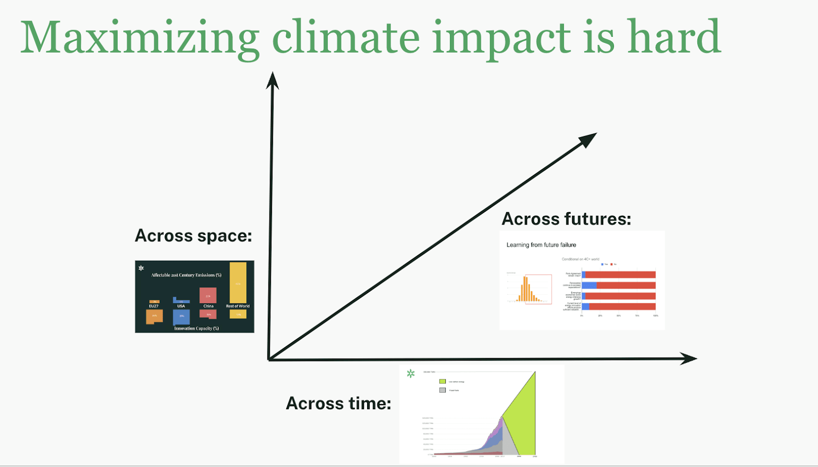
Rather, there are at least three dimensions along which to evaluate any action on climate and this means that the goodness of a particular action is not directly observable:
- Time: “What is the cumulative impact over time?” becomes
- Time & Space: “What is the cumulative global impact over time?” becomes
- Time & Space & Futures: “What is the cumulative global impact over time taking into account different ways the future could go and, relatedly, different marginal climate damage?”
Let’s tackle each layer in turn.
First, many of the best actions in climate that one could take will take years, sometimes decades, to fully materialize their effect. The best example to illustrate this is the dramatic cost decline and resultant diffusion of solar, which was the result of policies taken in the early 2000s. From an emissions standpoint, initial subsidies for solar looked terribly inefficient, one of the most expensive ways to reduce emissions one could conceive at the time. But there are few, if any, other actions that have had a similar long-run effect on global emissions. For forward-looking examples this disconnect between short-term and long-run consequences introduces very significant uncertainties.
Second, the effects of many actions are often not where an action is taken. Sticking with our solar example, it is safe to say that more than 95% of the emissions benefits of cost reductions of solar will not occur in the jurisdiction most responsible for them (Germany). Similar things could be said about electric cars (California), wind power (Denmark), and many other examples. The global diffusion of effects presents another layer of significant uncertainty, effects we need to grapple with and we should optimize for (having global effects is a good thing!), making answering the question of impact maximization harder.
Third, and most subtly, the effects of our actions might be more or less effective in different futures and they might be more or less important depending on the future we end up in.
For example, when heading into a future where geopolitical competition is severe we might be less optimistic about solutions that require strong international cooperation to be effective. What is more, solutions that would only work under those conditions of strong international cooperation will have most of their effects in futures where avoiding additional climate damage is less valuable because avoiding additional climate damage is less valuable at lower temperatures. Conversely, there are solutions that “hedge” against typical failure modes, that are robust or even particularly effective in futures where it matters most. We discuss this lots more here and, less technically, here if you are interested to learn more. For now, suffice it to say that these considerations – taking into account different future trajectories – are important, but also introduce significant additional uncertainty about the quality of different actions.
Bottom up: Thinking through enacting change
Another way to see these very significant uncertainties is much less big picture, and much more bottom-up.
Whenever evaluating whether to fund something the theory of change might look like something like this. (The particulars of the intervention do not matter here, what matters is that we are always moving through a path with many steps, each adding uncertainty along the way.)
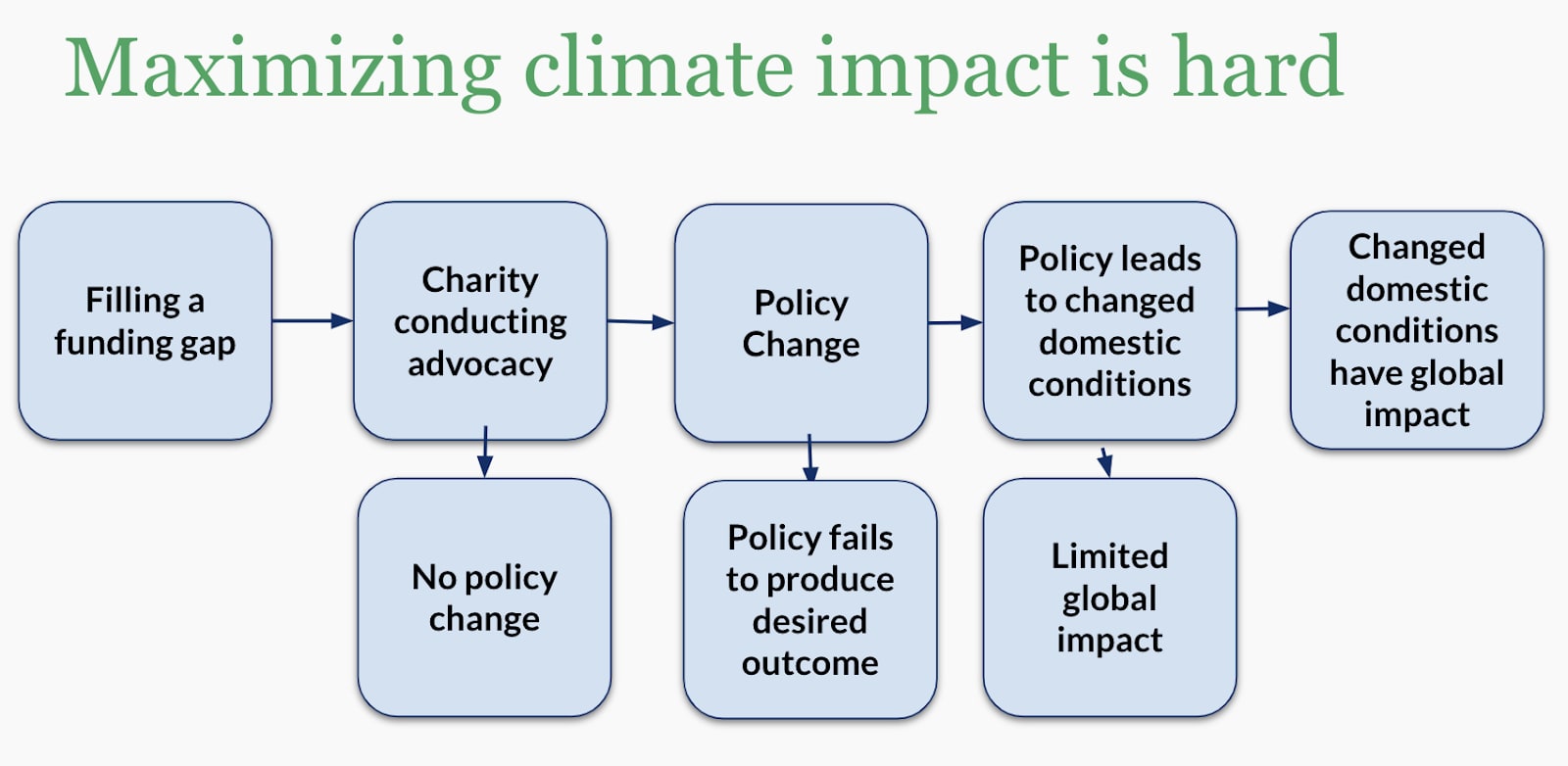
For example, (i) when we decide to fund something, we are uncertain about whether someone else would have funded it otherwise (reducing our counterfactual impact to zero).
Let’s say we funded it.
We are then uncertain about (ii) whether the work we funded will change policy and how much (even if we observe policy change, we do not know whether our funding was necessary!), (iii) whether that policy change will produce the desired outcomes domestically, and (iv) whether that will have meaningful global effects.
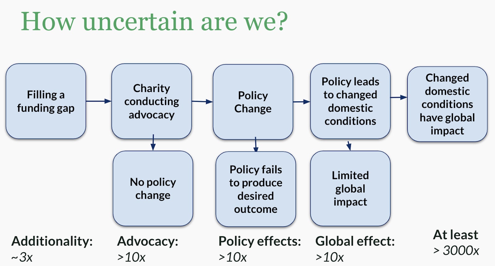
If we ask ourselves how uncertain we should be across all those steps even a quick guess reveals that our uncertainty about the effectiveness should probably be in the order of 1000s of times.
- Climate is a crowded space and we should generally never assume a funding additionality close to 1 (which would suggest certainty no one else would fund it). But is our chance of additionality 20% or 60%? This will often be hard to say (3x uncertainty).
- Tracing the impact of advocacy is inherently hard. The most successful examples are often examples where charities incubate ideas which are then owned by policy makers with no public record of impact. How effective a given effort is also depends strongly on the political environment (how good or bad did different interventions look before and after Senator Manchin decided to support what became the Inflation Reduction Act?). We should thus be honest that our uncertainty about how effective a given advocacy effort is should be at least 10x, probably significantly larger.
- Similarly, the impact of any given policy depends on the quality of implementation, features of the world we do not know before, as well as general political, economic and geopolitical conditions, to name a few. Again, an uncertainty of a factor of 10x seems conservative ex ante.
- Lastly, for promising actions, what really matters is the degree to which they have global and/or long-term consequences. Will a given technology diffuse globally? (innovation) Will a policy be widely adopted? (policy leadership) Will a given infrastructure investment really lock-in or lock-out a promising low-carbon trajectory for decades? (lock-in). These factors, again, are easily uncertain by more than an order of magnitude (10x).
Because these are steps along a sequential pathway of impact, multiplying these uncertainties is an informative way to think about the size of the total uncertainty about the specific impact (or, equivalently when taking into account cost) cost-effectiveness of any given funding uncertainty. In this case, this means we should be uncertain by a factor of at least around 3000x and this example is typical.
That, of course, is highly uncertain and makes questions such as “does this meet the bar for funding?” seem impossible to answer. A first reaction might very well be to consider this a futile exercise and shrug.
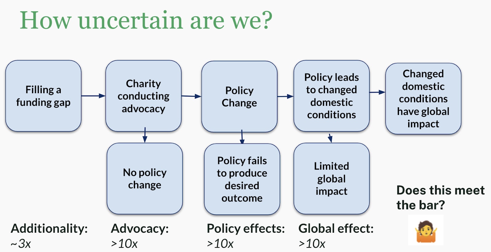
Should we just throw our hands up in the air?
[Slightly more detail, Lots of more detail]
One might say now: Let’s just throw our hands up in the air – we cannot say anything meaningful about the impact of different opportunities when things are very uncertain. We might as well treat everything as similarly good and worth doing.
We think this would be a huge mistake! To understand why, let’s first understand a bit more deeply why this is hard before outlining ways for how this could still be tractable.
There are two fundamental reasons that make this hard:
- (1) Uncertainties are very large and layered
- (2) Uncertainties are irresolvable on action-relevant timelines
The first is easy to see from the example above. There are four steps in the theory of change and each of them is (highly) uncertain.
If all the uncertainties are independent – meaning knowing how one would resolve tells us nothing about the others – we are right to multiply them which gives us an overall uncertainty of at least 3000, with four uncertainties layered on top of each other.
The second reason is more fundamental. These uncertainties are not resolvable on action-relevant timelines.
If we were in the business of evaluating direct delivery malaria interventions, this would be different. We could conduct or commission randomized-control-trials (RCTs) or other high-quality studies to narrow down the key uncertainties, hopefully allowing us to come out with a clear course of action.
But in climate the uncertainties are about long term processes, such as about the likelihood, duration, and effects of policy change, institutional change, and technological change.
Those are uncertainties we cannot avoid – if we go for certain things there is essentially nothing that looks even close to impact-maximizing – and that we cannot resolve on timescales that we can wait for.
This means we are stuck with the situation as is: one of very significant uncertainty. And so, should we just throw our hands up in the air?
No! We can make progress
[Slightly more detail, Lots of more detail]
Luckily, there are also some features of the situation we find ourselves in that make this a bit easier and we are going to exploit those as much as we can to make progress despite large uncertainty:
- (3) Uncertainties are often independent or their structure is understood.
- (4) Uncertainties often apply similarly to options we consider.
The first feature that makes this easier is that we often know something about the structure of uncertainty. For example, in many cases – as in the above example – the uncertainties are independent, with one uncertainty resolving not telling us anything about how other uncertainties might resolve. In this case, you can just multiply them out. While this does not reduce the uncertainty, it makes it cleanly representable. Another typical case is that while the uncertainties are not independent, we know how they relate to each other – for example, they are negatively correlated – allowing us to model them as such.
The second feature here is more subtle but also more helpful. The same or similar uncertainties often apply similarly to the different options that we're considering.
For example, we might be confused about whether to support a charity advancing alternative proteins compared to a charity advancing the decarbonization of cement.
We have lots of uncertainties with either option – how successful is advocacy usually? how much do early support policies matter? etc. – but there is a lot of shared structure to the uncertainties between those options.
Because of this, even though we will be very uncertain about the absolute cost-effectiveness, we can say meaningful things about relative effectiveness.
And that is really the bottom line here: Even though we can't really get a good grasp of absolute cost-effectiveness because that might be uncertain by a factor of 3000x or more, we can still say reliable things about relative impact. And, luckily, that is what ultimately matters, because we're trying to make the best decisions choosing between different options.
So, exploiting these two features makes it possible to get to credible comparative statements despite irresolvable ex-ante uncertainty on absolute impact.
The rest of this piece is using lots of visualizations and examples to bring these quite abstract points to life.
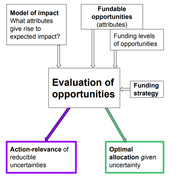
The Solution
Before we dive into a specific example to demonstrate, here is the big picture for how we think about solving this problem:
At a high level, we are building a suite of tools to bring to life our vision of credible high-impact grantmaking in the climate space. The tools we are building are always comparative, always represent uncertainty, and are meant to be jointly comprehensive – integrating key considerations that are relevant to evaluate a funding opportunity’s expected cost-effectiveness.
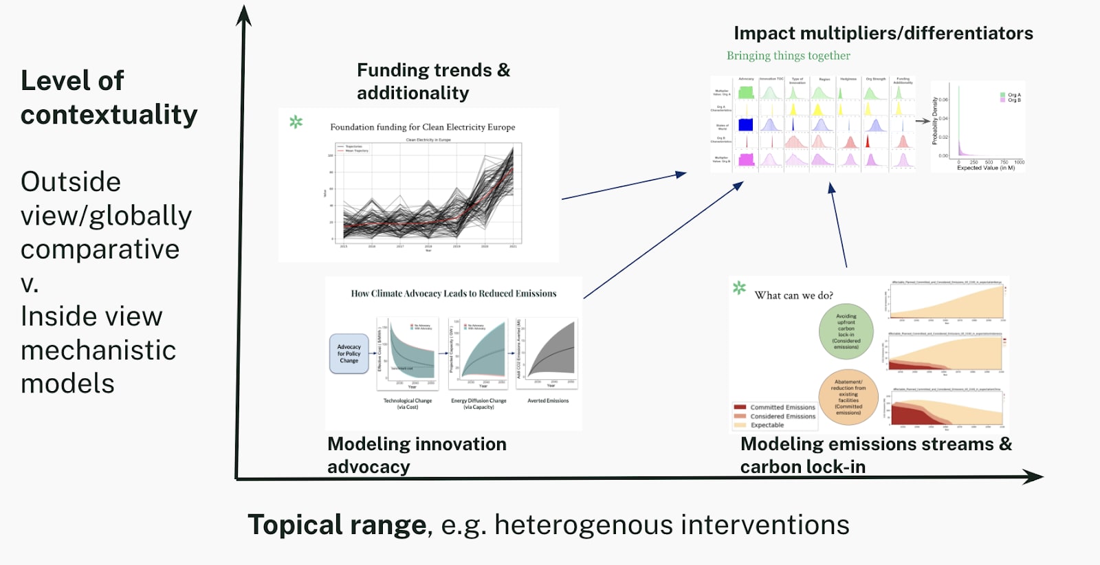
These tools vary in their level of abstraction and generality. At the most granular level stand mechanistic models that try to capture the essence of a relevant process, e.g. innovation advocacy, or specific carbon lock-in interventions. By their nature, these models are not general. At an intermediate level of specificity are tools that are general and inform a specific consideration, such as our modeling of funding trends and funding additionality. Finally, our overall impact model integrates the results of many different tools in a unified framework. This will all become clearer in the following demonstration.
A Demonstration
We will now demonstrate how we actually solve the problem outlined so far. In doing so, we highlight several of the “mechanistic” topic-specific tools that we have built over this past year as well as the overarching impact multiplier framework that we use in our integrated research and grantmaking agenda.
A realistic but stylized example
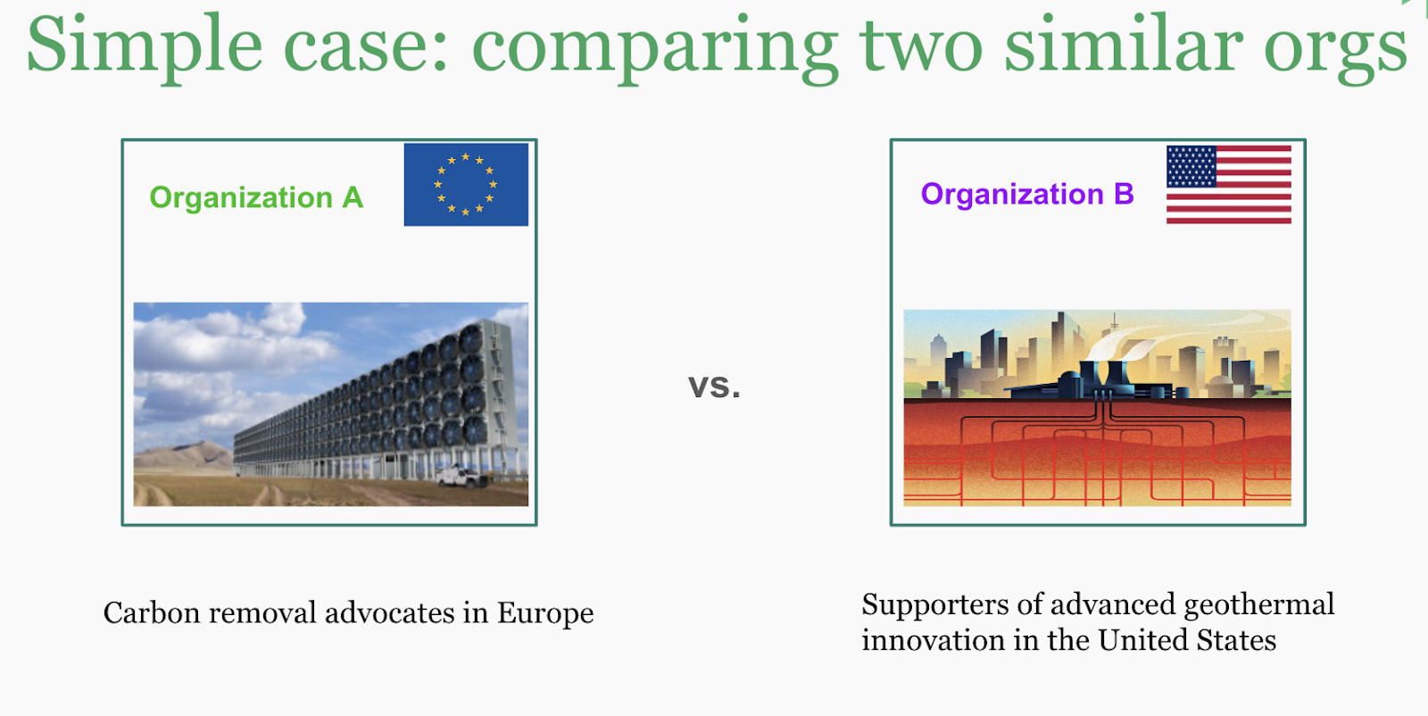
To describe the solution, we walk through a simple case study comparing two different organizations that, for simplicity (see “Solving at Scale”), both work in the innovation space as their theory of change. The two (mock-up) organizations that we look at are:
- Organization A: a carbon removal advocate located in Europe
- Organization B: a supporter of advanced geothermal innovation in the United States
While there are similar organizations existing, the examples here are intentionally fictional and the example is optimized for illustration, not representing a judgment on actual organizations.
In order to quantitatively compare the expected impact of these two organizations, we compare several distinct attributes between the two, as described in the subsequent section.
We ask ourselves “what are the essential attributes of these different funding opportunities we can fund?” and “what do we know about how these attributes are systematically related to impact?”. In this simplified example, we walk through seven different attributes, while in reality we usually consider more (see, “Solving at Scale”).
As the (famous) proverb goes “all models are wrong, some are useful”. This is very much true here. The point is not that a simplified model can capture all idiosyncrasies of a given funding opportunity, but that a simplified representation such as in the below framework is an approximation of reality that guides us in the right direction (in the same way as a map is a simplified model, but a good map helps us find the destination regardless despite not capturing all the details!).
How do we act? Advocacy
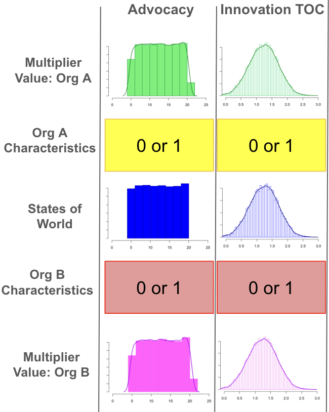
Throughout this walk-through, we will use the same visual language:
- In the center (middle row) we will represent states of the world, ways the world could be with regards to the impact-differentiating variable we consider. If the variable we considered were a regular dice, this would show a graph going from 1 to 6. Before we roll the dice, we are uncertain whether it will turn up a 1 or a 4 or a 6 and we think each of them is equally likely.
- In the rows above and below that, we represent the attributes of the given funding opportunity (organization), the degree to which a given organization leverages the described impact-differentiating mechanism (“the degree to which organization rolls this dice”).
- In the outermost rows, we represent how the state of the world and the attributes of the organizations interact.
The first characteristic we take into consideration is advocacy, by which we mean leveraging societal resources through philanthropy. We believe that there is an inherent impact multiplier from advocacy through our philanthropic work (see here and here why we believe this), but we have high uncertainty about the degree of the exact multiplier that advocacy results in:
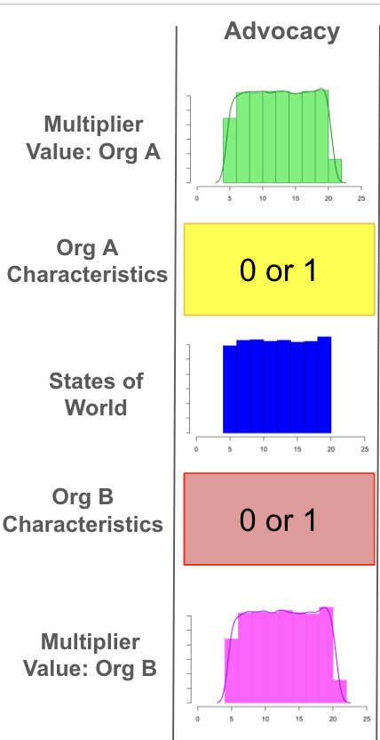
Distributions for the possible states of the world and organization-specific attributes for the advocacy multiplier.
In the distributions above, we plot the expected impact multipliers for each organization for the advocacy multiplier. Specifically, we plot the possible states of the world for advocacy in blue (middle plot) and the attributes of Organization A and B on advocacy in yellow and red, respectively. As shown by the blue plot, the uncertainty for the advocacy states of the world is fairly uniform, between 5 and 20 as an impact multiplier. The attributes for Organization A and B, plotted above and below the central distribution in yellow and red, respectively, are binary: either 1 or 0. In this case, we believe that both organizations leverage advocacy (i.e., organization characteristic = 1) and we have no reason to believe that organization A leverages advocacy more than organization B.
The final multiplier value of each organization for this variable is shown in the outermost distributions (green and purple), and is calculated by multiplying the state of the world (blue distribution) by the organization characteristic (yellow and red, respectively). Given that both organizations leverage advocacy equally, the multiplier value distributions for both are equal. Fundamentally, what we are expressing here is that we believe organizations leveraging advocacy to be more effective than those pursuing direct work.
What do we do? Theory of Change
We next consider the type of intervention, i.e., the theory of change that the organizations pursue. Given that both of the example organizations leverage innovation as their theory of change, we investigate what we expect the effect of such work to be not knowing anything else (we add contextual knowledge later!) than that the opportunities pursue this theory of change. To do so, we built out a tool that calculates the expected averted emissions resulting from advocacy for innovation policy change. The causal chain from advocacy to averted emissions is shown below:
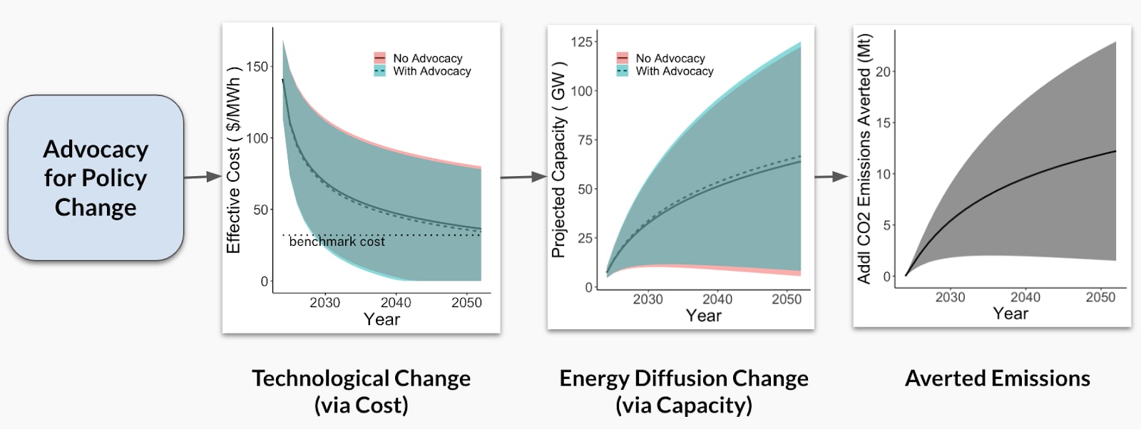
Process flow for Innovation TOC tool modeling the causal chain from climate advocacy to averted emissions
In this first step of the chain, our tool takes an input amount of advocacy dollars (what would be expected to be leveraged) that is meant for policy change, and determines the expected technological change of the underlying innovation as a result of this policy change. As shown by the first line plot, we assess technological change via cost decline curves. The plotted cost decline curves display the projected cost with and without advocacy-induced policy dollars, in the solid and dashed lines, respectively. As shown, the advocacy-induced scenario (dashed line, turquoise shading for region of uncertainty) occurs right below the line without advocacy (solid line, pink underlying shading for region of uncertainty) due to the accelerated cost decline curve over time that results from the additional advocacy dollars.
In the above plot, we continue our causal chain curves by adding the next plot: energy/ technology diffusion. We determine expected diffusion over time via projected capacity curves, which we calculate as a result of the cost decline curves from the previous step. Again, we represent capacity growth with and without advocacy, where the solid line (pink shaded region of uncertainty) indicates projected capacity over time for the no advocacy scenario and the dashed line (turquoise shaded region of uncertainty), which occurs just above the solid line, indicates projected capacity given advocacy.
Finally, given the difference between the advocacy and no advocacy capacity diffusion curves, we calculate the additional averted emissions due to advocacy-induced policy change. The calculated averted emissions are shown in the final plot below, with the gray shaded region representing our uncertainty at the 90% confidence interval. Given these projected averted emissions, the cost-effectiveness of advocacy ($ per ton) is measured by the cost of the initial policy dollars divided by the total (cumulative) additional tons of CO2 averted due to the advocacy intervention. As the averted emissions plot above has underlying uncertainty, so do our cost-effectiveness calculations.
We can therefore use the output of this tool to include the impact multiplier we expect from innovation as the intervention theory of change, as shown below:
Distributions for the possible states of the world and organization-specific attributes for the advocacy and innovation TOC multipliers.
As with our advocacy multiplier, the central blue distribution represents the expected possible states of the world for the impact multiplier from innovation. Notice, instead of a uniform distribution as we had expected with advocacy, our calculations for innovation suggest a normal distribution. Once again, the organization characteristics are binary (1 or 0) given whether or not the charity leverages this theory of change. In this particular example, since both organizations A and B work within the innovation theory of change space, both organizations do leverage this modifier variable (i.e., org characteristic = 1) and so we again have similar multiplier values for both organizations, as shown by the outermost (green and purple) distributions.
What do we act on?
We can also use our developed innovation tool to calculate the expected cost-effectiveness of policy across a variety of low-carbon technologies. Note, cost-effectiveness here refers to the additional mitigation induced due to policy dollars, as described in the causal chain above, not the cost-effectiveness due to the total cost of the technologies.
We then account for the expected cost-effectiveness across technologies in our modifier distributions. In the modifier distributions below, the blue states of the world distribution is the modifier distribution for the average innovation and the Organization A/B characteristics (yellow/red curves) refer to the relative cost-effectiveness of the target innovation compared to the average innovation. For example, we can compare the expected cost-effectiveness of the two technologies in our case study: direct air capture (DAC) and superhot rock geothermal (SHR). We plot the cost-effectiveness distributions for both of these technologies on the right side of the figure below, the results of which are then used for type of innovation modifier distributions on the left in green (for Organization A; DAC) and purple (for Organization B; SHR).
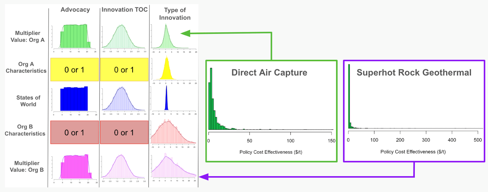
Left: Distributions for the possible states of the world and organization-specific attributes for the following multipliers: advocacy, innovation TOC, and type of innovation.
Right: Cost-effectiveness distributions for DAC and SHR technologies, which feed into the respective type of innovation distributions on the left.
As we can see, these distributions of expected cost-effectiveness look different between these two technologies. Both technologies have heavy tail distributions, however the SHR case displays higher values, as shown by the x-axis limits. This means that in some simulations there are some very high cost-effectiveness values for SHR, in which the intervention is not cost-effective, as it costs a lot of money to avert a single ton of CO2. This suggests that the expected cost-effectiveness for the DAC distribution is less uncertain than the SHR distribution, as shown by the narrower distribution for Organization A (yellow curve) than for Organization B (red curve) in the modifiers distribution.
However, we see that by far the greatest density of simulated values for the SHR distribution lies on the left-hand side of the plot, the highly cost-effective region. This means that, on average, advocacy for SHR policy interventions is likely to be highly cost-effective. The cost-effectiveness curve for DAC, on the other hand, has a less steep drop off than the SHR curve, where the simulated cost-effectiveness values are less densely concentrated far on the left side of the plot, thus suggesting an overall expected value that is less cost-effective.
To further understand which technology is more cost-effective on average, we divide out these two distributions to understand how often either technology is expected to be more cost-effective than the other. As such, we divide the DAC distribution by the SHR distribution. Our simulations show that SHR is expected to be more cost-effective than DAC over 90% of the time. As such, even though super hot rock geothermal has a wider distribution and more uncertainty, the vast majority of the time, it is more cost-effective to implement advocacy for superhot rock geothermal than it is for direct air capture.
While we only show two technology examples in this pairwise case study, our tool is capable of calculating the cost-effectiveness for any low-carbon technology.
Where do we act?
In addition to the specific technology, the next thing we want to take into account is where the intervention occurs and how this should affect our estimate of impact. For the case of innovation advocacy, we've built a tool that assesses innovation capacity in different jurisdictions. This work is a reanalysis based on 2021 ITIF data, in which innovation capacity calculations are assessed based on each jurisdiction’s:
- Capacity for early stage (e.g., R&D) innovation
- Capacity for late stage innovation and market readiness
- National commitments and international collaboration for low-carbon innovations
We significantly updated this data, integrating new policies (such as the IRA), and reflecting other relevant considerations (such as political uncertainty in the US affecting forward-looking estimates of innovation capacity, such as ours).
On the right in the figure below, we plot five different jurisdictions and their innovation capacity, as well as the respective 90% confidence intervals, given the three categories bulleted above. Given that Organization A is based in Europe and Organization B is based in the US, we specifically compare the innovation capacities for these two regions. In the bar graph below, we see that the EU and the US have the two highest bars, implying that they have similar expected innovation capacities. We moreover see high uncertainty for both jurisdictions, with a bit more uncertainty for the US than the EU, as shown by the error bars. While the EU and US have similar innovation capacities, we see large differences when comparing capacity of, for instance, the US versus India, as shown by the different bars below. These calculated innovation capacities, and underlying uncertainty, is then fed back into our respective Organization A and B multiplier distributions, as shown by the green and purple arrows below:
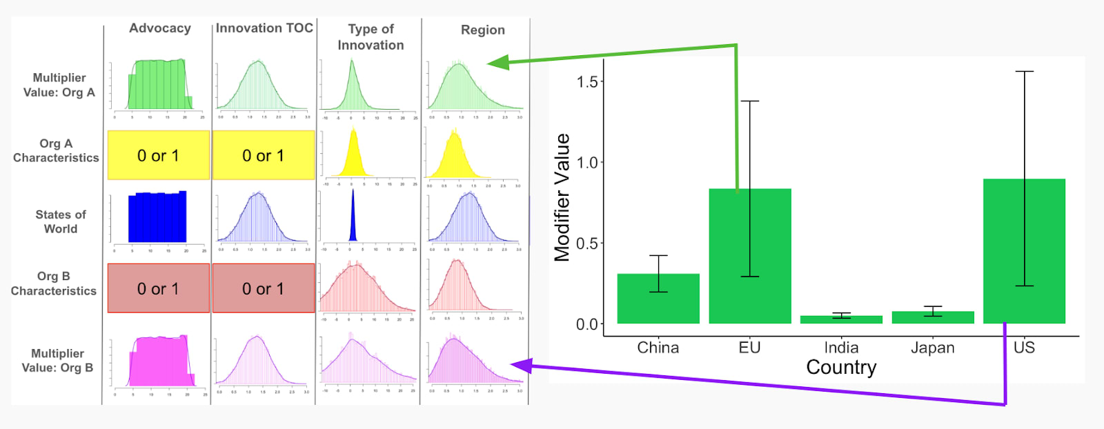
Left: Distributions for the possible states of the world and organization-specific attributes for the following multipliers: advocacy, innovation TOC, type of innovation, and region.
Right: Innovation Capacity across jurisdictions, including 90% confidence interval error bars. The innovation capacity for the EU and US are then fed back into the regional distributions of the left.
We thus use these calculated innovation capacities to inform our impact modifier distributions. Once again, we plot the possible innovation states of the world in blue (center distribution) and use yellow and red to represent the innovation capacity distributions for the EU and US, respectively. The final multiplied out distributions are plotted in green and purple; these distributions look similar due to the fact that the US and EU have similar innovation capacities. However, we can see that the purple distribution (US) is a bit more uncertain (i.e., wider) than the green (EU) distribution due to the fact that the calculated US innovation capacity has a larger confidence interval, as shown in the bar graph to the right.
This feature of the wider uncertainty, while sounding technical, represents something real and relatively straightforward – it is related to larger partisan and policy swings in political conditions in the US compared to the EU.
How robust and hedgy are our solutions?
[lots more here, somewhat less technical here]
The next characteristic that we want to account for in this analysis is how robust and hedgy these possible solutions are.
As discussed above (section on “Big Picture”) when optimizing across futures one important consideration is whether a given solution is robust to geopolitical, technological, climate and other macro conditions. Indeed, ideally solutions are not only robust, but “hedgy”, performing better in those worlds where it matters most (worlds that are both reasonably likely and damaging resulting in high expected climate damage). This is what we are trying to capture here (see the links above for more detail), though our quantification is more preliminary and, hence, more uncertain.
In our example, we note that carbon removal via direct air capture would require high coordination and willingness to pay given its cost point, which seems unlikely to be available in these types of high risk high climate damage worlds where it would be most useful. In other words, carbon removal via direct air capture appears as a solution with low “hedginess”. As such, we assign about 20th to 40th percentile hedginess to Organization A.
For Organization B, on the other hand, which advocates for clean firm power (e.g., geothermal energy), we expect that this type of energy would hedge against constraints on variable renewables. Given that we “know” that constraints to variable renewable diffusion are one of the clearest ways by which we end up in a future with high marginal climate damage, we allocate a 60 to 80th percentile hedginess to Organization B. This means that we think this intervention is among the 20-40th percent of most hedgy interventions.
We take these percentiles and apply them to our hedginess distributions for Organization A and B in yellow and red, respectively. For the states of the world distribution, hedginess is a binary variable – 1 or 0 – either it is leveraged or it is not. As shown, our overall multiplier distribution for Organization B (purple) has a higher overall expected hedginess value with greater uncertainty than the multiplier distribution for Organization A (green), given their different hedginess percentiles.
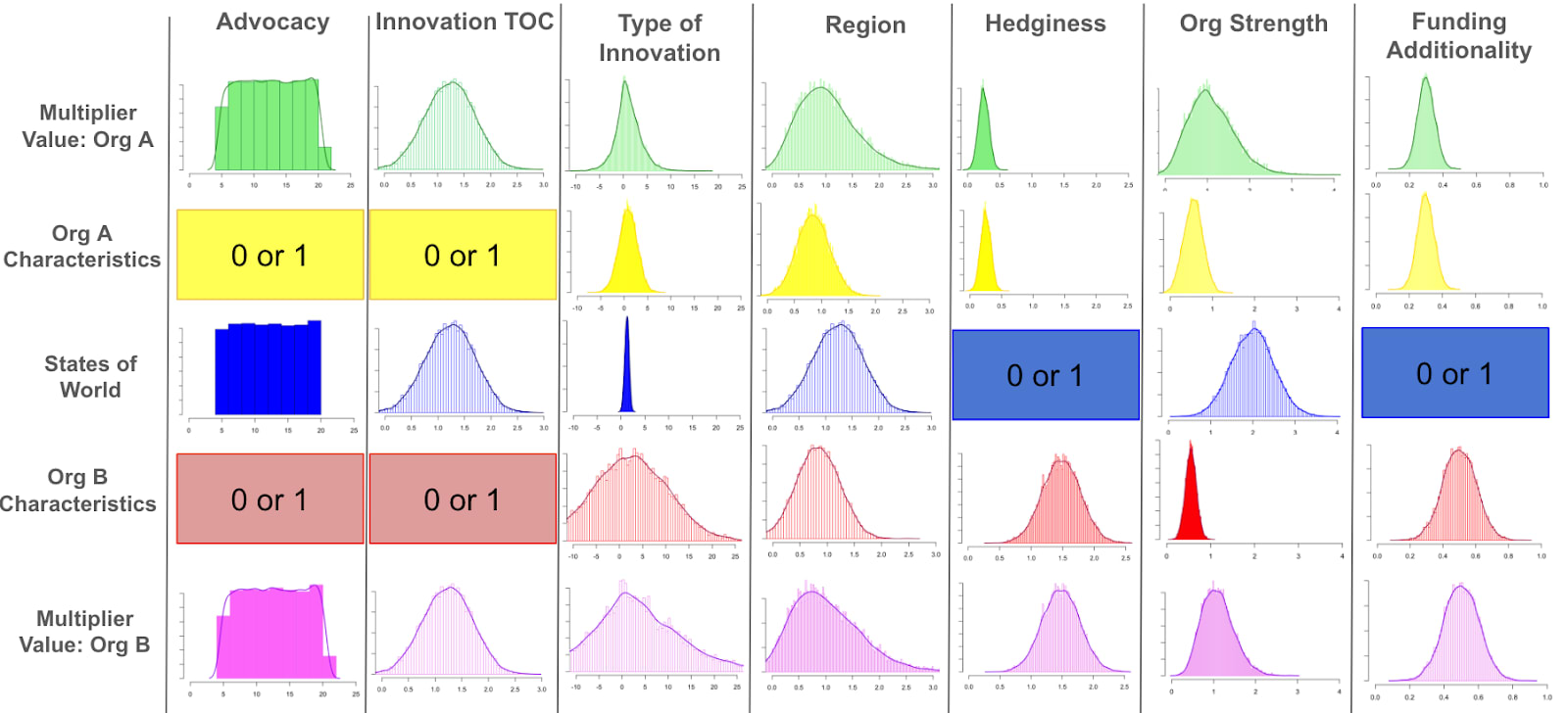
Distributions for the possible states of the world and organization-specific attributes for the following multipliers: advocacy, innovation TOC, type of innovation, region, and hedginess.
Who acts?
We next consider the strength of the organization when building our impact multiplier framework. We currently believe that organizations A and B are similar in expected strength, with some differences in their respective amount of uncertainty; e.g., the yellow distribution (Org A) is slightly wider than that of the red distribution (Org B).
The overall uncertainty is pretty large here, so if our goal were to identify precise absolute cost-effectiveness rather than relative cost-effectiveness, further research could likely narrow the uncertainty here.
Distributions for the possible states of the world and organization-specific attributes for the following multipliers: advocacy, innovation TOC, type of innovation, region, hedginess, and organization strength.
How additional is our funding?
Finally, we implement another tool that we have built out – calculating the probability of funding additionality for a given sector/region pair. Ultimately, we are interested in knowing how much funding is going into any given sector/region to determine whether or not a grant would be additional in this area.
To answer this question, we have built a Monte Carlo simulation that tracks and estimates trajectories for different sector/region pairs in the climate space. This uses data from ClimateWorks, but also includes additional information on individual and HNW giving, the steepness of funding influx, and the number of funders and grantees in a given space to estimate funding additionality (full model not shown here, as it is still being finalized).
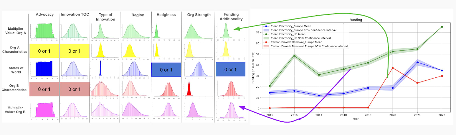
Left: Distributions for the possible states of the world and organization-specific attributes for the following all multipliers of interest.
Right: Funding trends for clean electricity and carbon removal in the US and EU, which are used to calculate funding additionality in the distributions of the left.
To apply this to our matrix of modifiers distributions, funding additionality for each sector/region is calculated based on these trajectories and used as the organization characteristics distributions (yellow and red) above. For the states of the world distribution, funding additionality is a binary variable – 1 or 0 – either it is leveraged or it is not. In the example above, Organization B (SHR in the US; purple) has a slightly higher expected funding additionality value than Organization A (carbon removal in the EU; green), however there is more uncertainty for Organization B funding additionality, as shown by the wider distribution.
An all-things-considered view
We then use each of these observed characteristics to calculate the expected value of each organization, where the expected value for organization A is the product of all of the green distributions on the top and for Organization B is the product of all of the purple distributions on the bottom.
This provides the answer to the question “given everything we know, what should we expect about the relative impact of the two options?”. In other words, what is our all-things-considered view based on the observed characteristics of the organizations and what we know about the climate philanthropy and action space.
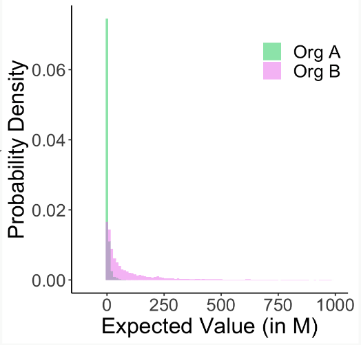
Total expected value distributions for Organizations A (green) and Organization B (purple)
In the figure above, we plot the distribution of simulated total expected values for Organization A (green) and Organization B (purple). As shown, the distribution for Organization A – carbon removal in Europe – is more densely concentrated on the left side, where the expected values are lower, than the distribution for Organization B – advanced geothermal in the US.
If we look at the specific simulated values, the average expected value for Organization B is 123 whereas it is only 3.7 for Organization A, about a 40x difference in expected impact. Moreover, we can see that Organization B has a heavier tail distribution, due to the underlying heavy tail modifier distributions for Organization B. One might say “Organization B is more hits-based” or, more precisely, with Organization B there is the potential for hits, outsized positive outcomes. Correspondingly, uncertainty in Organization B’s expected value is also higher than for Organization A.
This is an interesting outcome – one option looks on average 40 times better than the other – especially because it is derived from combining lots of individual pieces of relatively weak (uncertain) evidence.
One might reasonably say now that a 40x difference in impact is not meaningful (not really different from zero) in a context where overall uncertainties are in the 1000s. However, this would be mistaken because, as discussed above (Section “No! We can make progress”) a lot of the uncertainties apply similarly to the different options, leaving us far more confident in the impact differential than what the 40-to-1000s-ratio would suggest.
We can see this by plotting a graph like the below: Organization B outperforms Organization A when the above plotted ratio is greater than 1; in other words, when the expected value for Organization B is greater than the expected value for Organization A. As shown in the distribution ratio above, Organization B has a greater expected value than Organization A in 91% of the simulated cases.
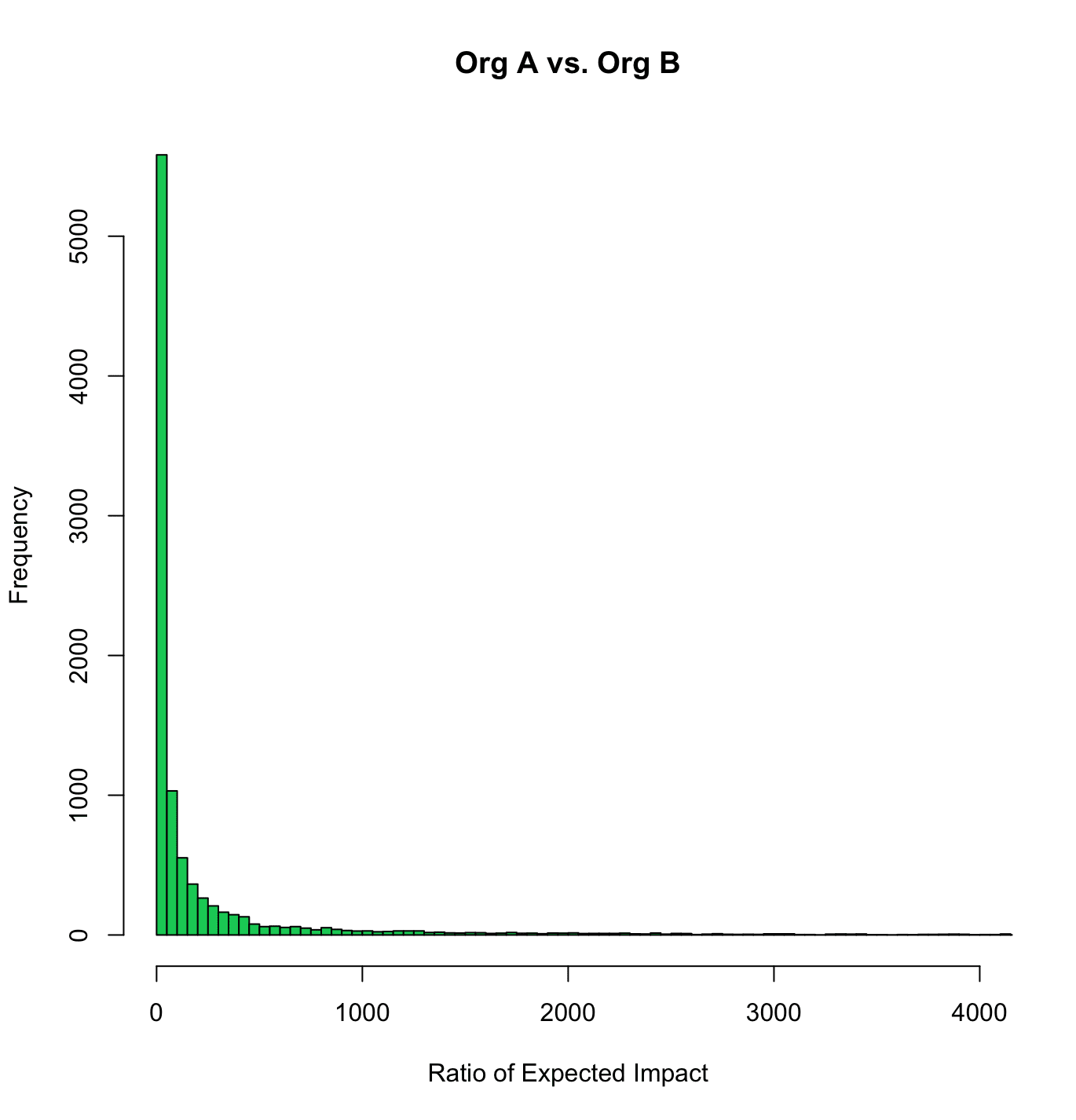
Expected value ratio for Organizations A vs. Organization B
This means that even though there is much more uncertainty of the exact expected value for organization B, we know that 91% of the time its expected value dominates over that of Organization A.
Thus, while uncertainties are often large, when combined they can still allow relative confident statements about impact differentials. Put differently, various forms of weak evidence conjunctively allow stronger relative statements.
Solving at Scale
Now that we have illustrated a concrete example, it is worth zooming out again and clarifying how this simplified example relates to a broader and more comprehensive research and grantmaking program – seeking to find and fund the best opportunities in climate.
To do so, we zoom out along three dimensions: First, we discuss the breadth of interventions we want to be able to compare – zooming out alongside interventions. Second, we discuss the set of impact-differentiating variables we consider in more complete cases – zooming out across attributes that we think are relevant to consider. Third, we discuss how this approach scales from a simple pairwise comparison to evaluating tens of organizations, providing quick but credible judgments about relative impact that can then be deepened in more specific analyses.
Scaling Dimension I: From similar cases to comparing across diverse theories of change
[A lot more detail on five of the six theories of change discussed here, the sixth – mitigating political risk will be discussed in an upcoming piece]
Until now we compared relatively similar things which we could have compared more mechanistically, e.g. directly within our innovation advocacy estimation tool. But, fundamentally, we need to be able to compare more broadly across different kinds of interventions that are driven by different theories of change that leverage varied impact multipliers.
This is for at least two reasons:
- The best opportunities might be found in very different “parts” of the intervention space so we need an integrated framework to compare these opportunities at a higher level of abstraction than those provided by “mechanistic” comparative tools closely modeled after specific mechanisms.
- Given the large uncertainties discussed throughout, and the conjunctive nature of impact (impact arising as a product of different variables) an” approach of only hierarchically drilling down (e.g. only choose the most promising theory of change, and only in the promising region, and with the most promising organization) is likely to miss some of the best opportunities.
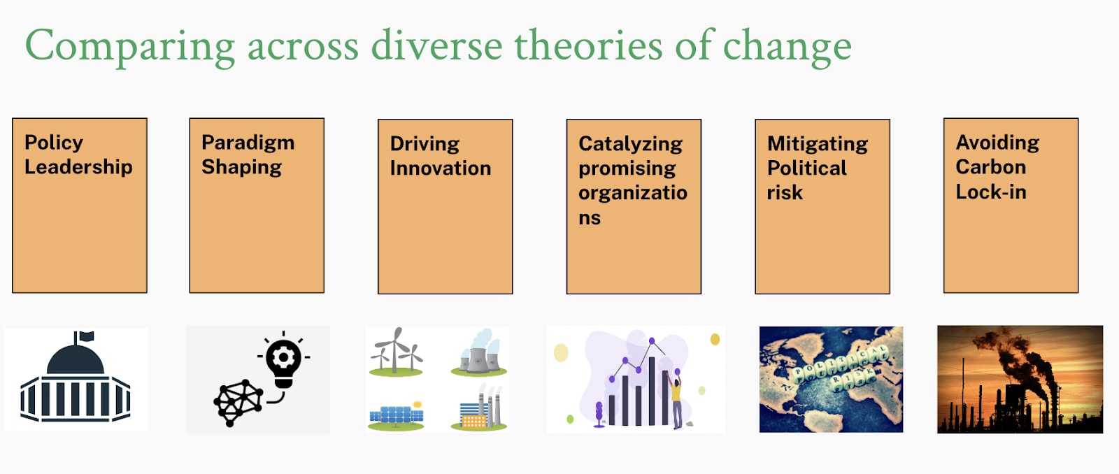
We currently have defined six different theories of change and are willing to consider all theories of change that have a plausible case at having an outsized impact. Our current belief is that a feature that gives rise to potential for outsized impact is the underlying feature of “trajectory change”, that relatively small changes in the world can have much larger consequences because they induce self-reinforcing dynamics or other path-dependent mechanisms translating small local changes into larger patterns. That is an idea underlying almost all of the theories of change we currently consider:
- Driving Innovation, accelerating the development and commercialization of low-carbon technologies through targeted advocacy aimed at improving innovation efforts in jurisdictions with high innovation capacity.
- Avoiding Carbon Lock-In, ensuring that long-lived infrastructure investments are as low-carbon as possible and that we pursue credible paths to decarbonize otherwise committed emissions, e.g. from young coal plants in emerging Asia.
- Catalyzing promising organizations, growing small organizations to scale enabling them to leverage climate philanthropy at large.
- Mitigating political risk, ensuring that there is robust support for the most important climate policies and that climate policy is robust to different partisan outcomes.
- Paradigm Shaping, introducing new ideas into the discourse that can shape policy and other action in the long run (in case this sounds abstract, see e.g. grant I here).
- Policy Leadership, advocating for policies in key jurisdictions that would have a chance to spread internationally.
In defining these theories of change, we can represent specifics while also combing them – through representation in our overall model – similarities that matter for all philanthropic interventions irrespective of their theory of change, such as funding additionality, hedginess, advocacy, and organizational strength.
For example, when we compare between interventions that drive technological innovation with interventions focused on policy advocacy to avoid carbon lock-in in emerging economies, we can leverage the knowledge about mechanisms of impact for both of these interventions: while what they do might be fundamentally different, we can apply the same considerations around funding additionality (for example, are interventions in emerging economies systematically less funded than high-income country interventions?) and organizational strength, while also honestly representing the heterogeneity of the work. Fundamentally, we believe that the grammar of impact – in particular, focusing on approaches that are neglected compared to potential and on mechanisms that can leverage large resources and drive trajectory change – is more general than often assumed and that comparing different interventions, while certainly difficult, need not invite fatalism.
Scaling Dimension II: Comprehensive impact differentiators
[Slightly more detail]
Another way in which this example was simplified is that it only considered a subset of the variables we include when characterizing a funding opportunity.
Of course, considering only a subset of variables can lead to wrong conclusions – in particular when one thinks that impact arises as a product of different considerations (“effectiveness is a conjunction of multipliers”) so that the omission of impact-differentiating variables can lead to misleading results.
For this reason, we think it is important to be comprehensive in the variables considered and to consider at least the following ones for every funding opportunity. They fall into three broad buckets, characterizing the pursued intervention, additionality, and organization, respectively.
Importantly, characteristics of the intervention or characteristics of the organization are both quite partial and only considering them can be quite misleading: when only considering an intervention, we know nothing about the strength of organizations in this space, nor about the impact of more funding. When only considering an organization’s attributes such as observable track record or the team’s strength, we are throwing away lots of information about the relative promisingness of different interventions and the degree to which strengthening such interventions would be additional.
- Theory of Change/Intervention
- Theory of Change – what are the characteristics of the pursued theory of change?
- Robustness and hedginess – how robust and hedgy are the pursued interventions?
- Additionality
- Funding - what are funding dynamics right now and what should we conclude from this about our funding being additional?
- Neglectedness - how much has already been tried and what should we assume about the effectiveness of new projects based on this?
- Activity - how many other actors are pursuing similar initiatives and how should this affect our estimate of impact?
- Policy - how many of the averted emissions are additional to what is already mandated / locked in by existing policy?
- Org-specifics
- Organizational Strength - how capable is the organization?
Note that we see this as a minimal specification and in practice will usually specify additional variables if we have other systematic information that we can exploit to understand differences in expected impact across options – for example, the technological heterogeneity included in our demo above.
Scaling Dimension III: From pairwise comparisons to mapping the space
Finally, the stylized pairwise comparison, is of course, not what we are ultimately after. Rather than comparing two cases we are building the analytical infrastructure to compare tens of options at the same time.
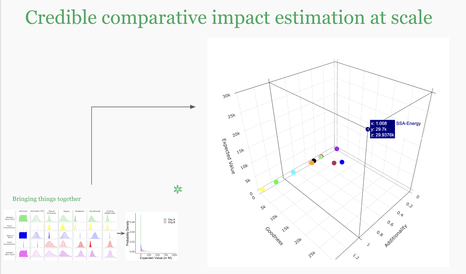
Ultimately, this is an N-dimensional space (where N = number of impact-differentiating variables) that cannot be easily visualized in 3D, so the above – aggregating into variables around additionality and goodness, with their product the expected impact – is merely a mock-up to convey intuition.
We are currently experimenting with a Grant Opportunities Idea questionnaire where interested charities and others can submit ideas for consideration, ideally in 1 hour or less (for an organization used to submitting grant ideas). The goal of this process is to collect all relevant information to quickly form initial views.
Through the full representation of expected impact and the surrounding uncertainties we are integrating our grantmaking and research process with the overall impact model producing both optimal grant allocations given current beliefs about impact as well as identifying key uncertainties for research, identifying which uncertainties’ resolution would most likely change decisions and should thus be prioritized (more detail here).
Conclusion
In this piece, we tried to characterize the problem we face when making claims about expected impacts in a high-uncertainty environment such as climate philanthropy.
We outlined that while this presents fundamental problems to confident claims of absolute cost-effectiveness, luckily we are in a better position regarding the question that matters for climate philanthropists – making the right choice between different options, i.e. choosing the relatively better options.
With our illustrative example we demonstrated how we currently think about tackling this problem, introducing a suite of tools of varying granularity and generality along the way. We then discussed how this stylized example generalizes to more realistic cases, where we consider a wider set of impact-differentiating variables (including diverse theories of change) and move from pairwise comparisons to comparisons of portfolios and tens of organizations.
This is all work in progress and we will update this note as we continue to develop our thinking and tooling on these questions and are looking forward to any feedback.


Thanks for sharing your thinking in a detailed and accessible way! I think this is a great example of reasoning transparency about philanthropic grantmaking, and relevant modelling.
How are you thinking about adaptation to climate change (e.g. more air conditioning)?
I do not think this is correct. If the component uncertainties are independent, the overall uncertainty will be narrower than the suggested by the product of the component uncertainties. If one gets a relatively high value in the 1st multiplier, one will tend to get a relatively lower value in the 2nd due to regression to the mean (even if the multipliers are independent). If the multipliers were perfectly correlated, then the overall uncertainty would be the product of the component uncertainties.
If Y is the product of independent lognormal distributions X_1, X_2, ..., and X_N, and r_i is the ratio between the values of 2 quantiles of X_i (e.g. r_i = "95th percentile of X_i"/"5th percentile of X_i"), I think the ratio R between the 2 same quantiles of Y (e.g. R = "95th percentile of Y"/"5th percentile of Y") is e^((ln(r_1)^2 + ... + ln(r_N)^2)^0.5). For multipliers whose 95th percentiles are 3, 10, 10 and 10 times the 5th percentiles, the 95th percentile of the overall multiplier would be 62.6 (= e^((ln(3)^2 + 3*ln(10)^2)^0.5) times the 5th percentile. This is much smaller than the ratio of 3 k you mention above, but actually pretty close to the ratio of 40 between the all-things-considered expected value of organisations A and B!
As a side note, if all multipliers have the same uncertainty r_i = r, and are:
This might be a sensible reality check. However, I would say we should conceptually care about E("cost-effectiveness of A")/E("cost-effectiveness of B"), not E("cost-effectiveness of A"/"cost-effectiveness of B"), where E is the expected value.
How do you think about adaptation?
Do you have any thoughts on applying a similar methodology and developing analogous models for other areas where there is large uncertainty? I think it would be great to do for AI, bio and nuclear what you did for climate. Have you considered doing this at Founders Pledge (potentially with funding from Open Phil, which I guess would be more keen to support these areas rather than climate)?
I would also be curious to know whether you have tried to pitch your approach to non-EA funders, potentially even outside philanthropy. There is lots of non-EA funding going to climate, so it would be good if more of it was allocated in an effective way!
Hi Vasco,
Thanks for your thoughtful comment!
It took me a while to fully parse, but here are my thoughts, let me know if I misunderstood something.
I/ Re the 3000x example, I think I wasn't particularly clear in the talk and this is a misunderstanding resulting from that. You're right to point out that the expected uncertainty is not 3000x.
I meant this more to quickly demonstrate that if you put a couple of uncertainties together it quickly becomes quite hard to evaluate whether something meets a given bar, the range of outcomes is extremely large (if on regression to the mean the uncertainty in the example goes to ~40x, as you suggest, this is still not that helpful to evaluate whether something meets a bar).
And if we did this for a realistic case, e.g. something with 7+ uncertainties then this would be clear even taking into account regression to the mean. In our current trial runs, we definitely see differences that are significantly larger than 40x, i.e. the two options discussed in the talk do indeed look fairly similar in our model of the overall impact space.
II/ In general, we do not assume that all uncertainties are independent or that they all have the same distribution, right now we've enabled normal, lognormal and uniform distributions as well as correlations between all variables. For technological change, log normal distributions appear a good approximation of the data but this is not necessarily the same for other variables.
III/
"However, I would say we should conceptually care about E("cost-effectiveness of A")/E("cost-effectiveness of B"), not E("cost-effectiveness of A"/"cost-effectiveness of B"), where E is the expected value."
Yes, in general we care about E(CE of A/CE of B). The different decomposition in the talk comes from the specific interest in that case, illustrating that even if we are quite uncertain in general about absolute values, we can make relatively confident statements about dominance relations, e.g. that in 91% of worlds a given org dominates even though the first intuitive reaction to the visualization would be "ah, this is all really uncertain, can we really know anything?".
IV/ The less formalized versions of this overall framework have indeed already influenced a lot of other FP work in other cause areas, e.g. on bio and nuclear risk and also air pollution, and I do expect that some of the tools we are developing will indeed diffuse to other parts of the research team and potentially to other orgs (we aim to publish the code as well). This is very intentional, we try to push methodology forward in mid-to-high uncertainty contexts where little is published so far.
V/ Most of the donors to the Climate Fund are indeed not cause-neutral EAs and we mostly target non-EA audiences.
Thanks for the clarifications, Johannes!
I meant we should in theory just care about r = E("CE of A")/E("CE of B")[1], and pick A over B if the expected cost-effectiveness of A is greater than that of B (i.e. if r > 1), even if A was worse than B in e.g. 90 % of the worlds. In practice, if A is better than B in 90 % of the worlds (in which case the 10th precentile of "CE of A"/"CE of B" would be 1), r will often be higher than 1, so focussing on r or E("CE of A"/"CE of B") will lead to the same decisions.
If r is what matters, to investigate whether one's decision to pick A over B is robust, the aim of the sensitivity analysis would be ensuring that r > 1 under various plausible conditions. So, instead of checking whether the CE of A is often higher than the CE of B, one should be testing whether the expected CE of A if often higher than the expected CE of B.
In practice, it might be the case that:
How do you think about adaptation (e.g. economic growth, adoption of air conditioning, and migration)? I forgot to finish this sentence in my last comment.
Note E(X/Y) is not equal to E(X)/E(Y).
Thanks, Vasco, for the great comment, upvoted! I am traveling for work right now, but we'll try to get back to you by ~mid-week.