I would like to thank David Thorstadt for looking over this. If you spot a factual error in this article please message me. The code used to generate the graphs in the article is available to view here. 

Introduction

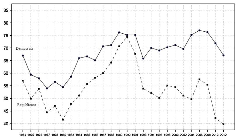
Say you are an organiser, tasked with achieving the best result on some metric, such as “trash picked up”, “GDP per capita”, or “lives saved by an effective charity”. There are several possible options of interventions you can take to try and achieve this. How do you choose between them?

The obvious thing to do is look at each intervention in turn and make your best, unbiased estimate of how each intervention will perform on your metric, and pick the one that performs the best:

Having done this ranking, you declare the top ranking program to be the best intervention and invest in it, expecting that that your top estimate will be the result that you get. This whole procedure is totally normal, and people all around the world, including people in the effective altruist community, do it all the time.

In actuality, this procedure is not correct. The optimisers curse is a relatively simple mathematical finding, first coined in this paper from Smith and Winkler, that proves that in many normal situations such a procedure is overwhelmingly likely to:

1. Overestimate the impact of the top intervention.
2. Bias your selection towards more uncertain interventions.

These effects can be small, or they can be drastic, depending on the interventions you are investigating. In general, the bigger the uncertainty in your estimations, the more worried you should be about the curse.

In this article, I will do my best to explain what causes the optimisers curse, using a toy model. I will demonstrate one solution to it, and describe how Givewell has reckoned with the curse in their charity evaluations.

I will do my best to make this accessible and understandable to everyone, even if you aren’t super mathy.

The optimisers curse explained simply

The optimiser's curse is a relatively simple mathematical result, first coined in 2006 in this paper in the journal of Management Science. It is closely related to the winners curse in auctions, and has some similarities to data dredging and regression to the mean in scientific contexts.

The key to the optimiser's curse is the simple fact that the evaluations of each intervention are not being made by omniscient gods. Anytime you make an estimate, you are forced to gather evidence, make assumptions, make calculations, and apply your own judgement to the estimate. At any stage you can make a mistake, or the sources you use could make a mistake, or you could be misled by the noise of an experimental trial.

All this means is that your estimate of an intervention's effectiveness will always be different from it’s actual effectiveness. It could end up being an underestimate, or an overestimate. If you are good, the magnitude of the error will not usually be that bad, but the more interventions you look at, the more likely it is that you’ll make a big error somewhere.

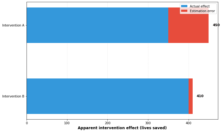
Then we add ranking in. In reality intervention A might save 350 lives, and intervention B might save 400 lives, but if you overestimate intervention A by a 100 lives and intervention B by only 10 lives, it will look like the better option, and you will pick it over intervention B. You will then expect it to save 450 lives, and be 100 lives too optimistic. The overall effect is that your top estimates will have an upward bias, even if every individual estimate in isolation is unbiased:

The other finding is that this advantages more uncertain causes. A grounded intervention that is well evidenced will have a smaller magnitude of error, on average, than a speculative intervention. The result of this is that the speculative intervention gets a better chance at a “high roll”, where it is massively overestimating, allowing it to jump much higher in the rankings than it deserves. In the graph above, the reason that intervention B appears superior to intervention A may be due to it being r.

This is the basic explanation of the optimiser's curse. In the next section, I want to demonstrate the curse in a more practical sense, using a toy model.  

 Introducing a toy model

In our model, we pretend we are a charity evaluator, investigating the lives saved per million dollars for a number of different charitable interventions. We decide to investigate and evaluate different interventions for their effectiveness.

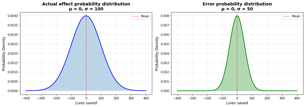
In this model, we will model the actual effect as sampled from a normal distribution, with mean of 0 lives saved and a standard deviation of 100 lives.  We then model the error for each intervention as sampled from a different normal distribution, with mean 0 and standard deviation of 50 lives.

Of course, actual charities evaluation is a lot more messy than this, but this simple model will suffice for demonstrating the curse in action. Here are the probability densities for our samples:

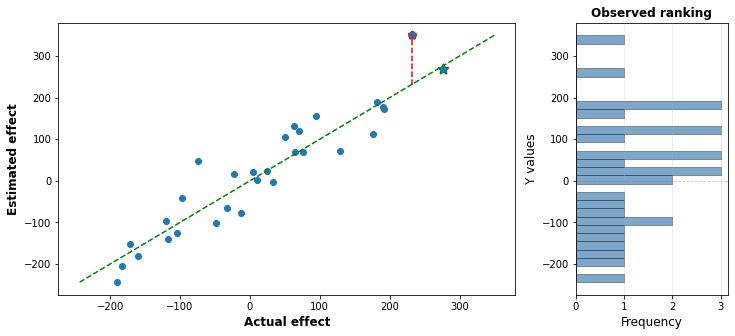
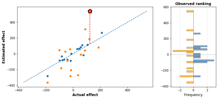
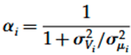
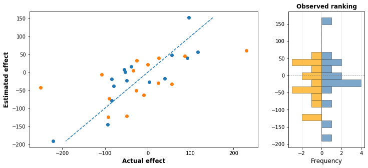
We investigate 30 interventions, grabbing a sampled actual effect and a sampled error, and adding them together to produce an estimated effect. I simulated this in python and produced the following graphs:

 On the left side, each dot is plotted with it’s actual intervention effect on the x-axis, and the estimated effect on the y-axis. The right graph shows what the actual estimator see: a straight ranking of the effectiveness of each intervention.

The green line in the middle is the line of accuracy: If the evaluators were perfect then the estimated effect would be the same as the actual effect, and every dot would fall on the line. But the evaluators are not perfect: some of the time they underestimate the effect, making the dot fall over the line, and sometimes they overestimate it, making the dot fall below the line.

Of course, the evaluators don’t see the “actual effect” part of the graph. All they see is the estimated effect, which is shown in a histogram on the right. In this case, it appears that the point marked with the red pentagon is the top charity.

But that’s not actually true: the top charity is just the rightmost point in the graph, marked here with a green star. In the estimates, it looks like the red point saves 50 more lives than the green point: in reality, it saves like 20 less lives, but it had a lucky draw on the error that made it appear better.

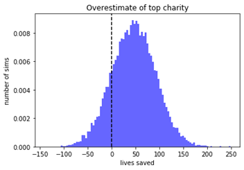
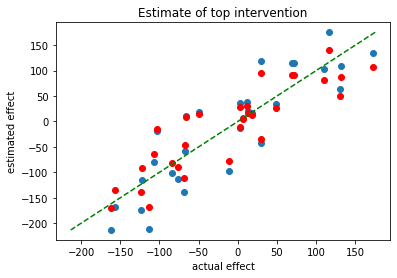
Now, that was just one simulation: if you run it again you will get different results. I ran this simulation ten thousand times, and stored how much of an overestimate you got from picking the top charity each time. It’s graphed below:

We can see that in the median case, the number of lives saved is an overestimate by about 50 lives. From other methodology, I found that this is generally around a 25% overestimate, compared to the actual value. Thus, in our toy model, the optimizers curse is vindicated.

The magnitude of the overestimate will increase if you increase the range of errors, or if you increase the number of interventions that are compared.

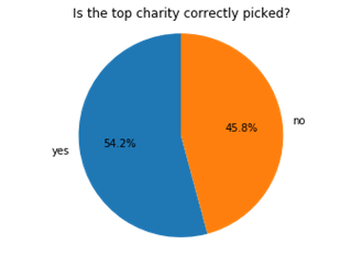
Now, what about the ordering of the charities?Under these conditions, the top charity is actually correctly picked a narrow majority of the time, and most of the time when it isn’t, the winner is in the top 3.

 So this doesn’t particularly change your decision procedure: if you want to maximise gains you should still pick the top charity, even though theres a decent chance it’s not the actual top one. This does recommend applying extra scrutiny to all the top charities, as the ordering may have been affected by error.

Introducing speculative interventions

 The far more interesting results come when you drop the assumption that all the interventions have the same level of uncertainty.

In the following simulation, I introduce another type of intervention, which I colour in orange. The true effects of these interventions are sampled from the same source as the blue ones (ie, they are no better on average), but their errors have a spread that is 4 times as large. We will call this the “speculative” type of intervention, and we will call our original type of intervention the “grounded” type.

The following graph shows what happens in one simulation, where 15 interventions are speculative and 15 are grounded:

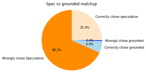
As you can see, the speculative interventions have a much wider range of estimates than the grounded interventions, because there is more room for error in either direction. As a result, when ranking the charities, it appears that the top speculative charity is almost twice as good as the top grounded charity. But this is a pure, error-based illusion. In reality, the top charity is a grounded one, but the speculative charity was just helped along by a very large error in it’s favour.

After running this simulation ten thousand times, we can compare the strategies. If you take the top estimated speculative charity, and the top estimated grounded charity, what happens if you just naively pick which is higher? Here it is:

93% of the time, the speculative cause is chosen, and the majority of time, this is actually the wrong chose.

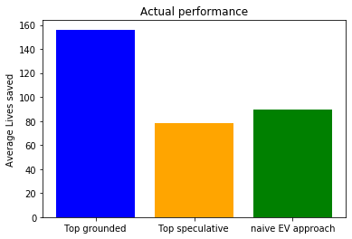
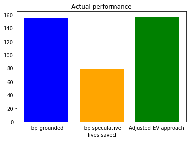
How does this get reflected in the actual performance? In the next set of simulations, I kept track of how many actual lives get saved for three strategies: investing in the top grounded intervention, investing in the top speculative intervention, or investing in whatever the top charity in the evaluation is. Here are the results:

That’s right, in terms of average lives saved, the winning strategy of the three here is to ignore the speculative causes entirely, and just invest in the top grounded intervention. This saves nearly twice.

This actually makes a lot of sense, when you think about it. Both the grounded and speculative causes have similar actual effectiveness, but in the case of the grounded interventions, you get much more useful information out of the evaluation and ranking process.

This is a mathematical demonstration that, in our simple model, an approach of naively investing in the top apparent EV intervention is straight up wrong. 

Note that in this toy model, both the speculative causes and the grounded causes are modelled as having the same mean and standard deviation of true effectiveness. You will get different results if these values are different. This toy model does not prove that all speculative causes are better than grounded ones: you can be extremely certain about how many lives you will save by buying yourself an Xbox (0), but that does not mean it is a better use of funds than buying malaria vaccines for people in extreme poverty.

A simple bayesian correction

So, how to we correct for the optimizers curse? In this article I will show the solution from the original optimisers curse paper by Smith and Winkler. This solution has been discussed before, but I was unable to find anyone actually implementing it in a toy model. This is surprising, because the math involved is actually incredibly simple.

Here is the equation from the original paper:

This corresponds to the following process:

1. Have a prior guess for the effectiveness of an intervention (${\mu }_i$) In our case, the natural choice is that the intervention does nothing.
2. Do all your intervention evaluation, to get your estimated value of the intervention ($V_i$).
3. Analyse the degree of uncertainty in your estimates and use that to determine a deweighting factor (${\alpha }_i$)
4. Using these two numbers, you then make a final estimate $v_i$ which is a weighted average of your prior and your calculated value.

They also detail an equation for how to determine the deweighting factor alphai:

The key parameters here are ${\sigma }_{\mu i}$ ,the standard deviation or spread of your actual interventions, and  ${\sigma }_{Vi}$ , the standard deviation or spread of your errors.^[1] In the equation, the ratio of these two spreads is squared.

I want to emphasise that it’s the ratio of these spreads that matters, so it’s not as simple as deweighting causes in proportion to their uncertainty: if intervention class A is twice as uncertain as intervention class B, but the actual effects of intervention class A are twice as spread out, then they should be deweighted by the same amount.

In our grounded intervention case, the spread of interventions is 100, and the spread of errors is 50. The ratio is therefore 0.5, which we square to get 0.25, and plug in to get a deweighting factor of 0.8.

This is applied to each in turn. So, for example, an intervention which gets an estimated effectiveness of 250 lives would get get deweighted, to produce a final estimate of 250*0.8 + 0*(1-0.8) = 200 lives.

The results are a bit more squished, compared to what you’d expect. But remember, this is taking into account the effect of the whole selection process. And if we repeat our earlier analysis with the adjusted estimates, we get the following after ten thousand simulations:

We can see that it basically worked perfectly: with this adjustment we are exactly as likely to overestimate as underestimate the effectiveness of the top charity.

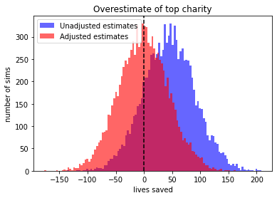
The difference is even more stark if we apply the correction to the extra speculative interventions from earlier. In this case, the spread of errors is 200, whereas the spread of actual interventions is only 100, leading to an alpha of 1/(1+(200/100)^2) = 0.2

Using 30 interventions, and 10 thousand runs, we can see that the speculative intervention greatly overestimates the lives saved, but applying the correction drops it down to zero.

Now, if we repeat our experiment from earlier, but apply our deweighting calculation, the grounded interventions are multiplied by 0.8, whereas the speculative are multiplied by a factor of 0.2:

This means that a speculative charity has to score four times as high on estimated effectiveness to be treated as equal to a grounded intervention. If the uncertainty increased further, the approximate rule would be that increasing the uncertainty by a factor of 10 causes the deweighting factor to drop by a factor of 100.

Here is one result for our grounded and speculative interventions, adjusted according to the formula:

We can see that the adjustment puts the spread of values between speculative and grounded interventions much closer together.

Now, when we run a few thousand simulations and compared approaches, the adjusted EV approach now gives the best overall performance:

Note that this doesn’t actually affect the effectiveness of picking out the top grounded or speculative intervention. This is because the adjustment doesn’t reorder interventions that have the same level of uncertainty. But now the adjusted expected value approach is performing better than either result.

The success of the grounded interventions reflects the fact that the best estimated grounded intervention really is better, on average, than the best estimated speculative intervention.

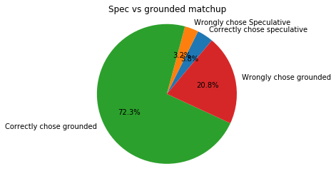
We can also look at how this affects choice between speculative and grounded charities:

So now, 90% of the time we are picking the grounded charities. This may seem unfair, but we are choosing correctly 75% of the time, which is way better than before where we were choosing wrongly 70% of the time. The fact is, in this situation the top grounded intervention really is the better choice most of the time, because the lower noise allowed us to do a better job at picking out the better grounded interventions.

Obstacles to simple optimizer curse solutions.

So, have we solved the optimizers curse here? Just guess at the parameters for the correction equation and then plug them in, and deweight everything by those factors?

Of course not. It’s easy to do well in a toy model because we know all the information, and everything is behaving in a nice, clean, predictable way. But in reality there are often significant obstacles. I will focus on the difficulty of doing this for charity effectiveness.

1. How do you estimate the spread of true effectiveness?

In reality, you are never going to see the actual effectiveness of an intervention, only the estimated effectiveness. So it’s going to be tricky to back-determine the spread of actual intervention effectiveness, when the spread you see is a mix of true difference and errors.

Ideally, you would have high quality data showing the actual effect of a variety of interventions, perhaps as a result of doing controlled experiments. However any situations where you have this is going to be a case where uncertainty is quite low anyway. If we are discussing a messy question like “how many lives does this charity save per dollar”, evaluations are difficult and costly.

2. How do you estimate the spread of errors?

This is a similar problem to the previous point: we don’t see the “true” spread of errors either.

Ideally, you would have a reliable database of predicted effectiveness vs actual effectiveness, but we run into the same issues as before: in cases where we have high quality data, the uncertainty is not that large anyway.  

3. How do you account for correlated errors?

All the demonstrations in my toy model where assuming that the error in each case is uncorrelated: this is not true in practice. Many similar interventions will share sources of error that affect both in the same way.

According to the paper, correlation reduces the magnitude of the optimizers curse, so if you assume no correlation you will end up overcorrecting for the optimizers curse.

4. How do you account for distribution shapes?

I’ve modeled this as a normal distribution, but is this actually the case? The nature of our selection process makes the shape of the distribution pretty important, because it’s the most extreme cases that are generally important. For example, if the distribution for errors is long-tailed, that should increase the magnitude of the curse, whereas if the distribution for the actual interventions is, it would decrease it.

5. How do you account for extra scrutiny after the initial analysis?

There is a much more well-known cousin to the optimizer's curse known as  “regression to the mean”. This is a well established statistical effect where initially extreme findings will end up dropping in magnitude when subject to follow-up studies.

A similar effect is likely to occur here: if you take the top interventions and subject them to increased scrutiny and follow-up studies, you will expect them to drop in estimated effectiveness over time, as errors get spotted and good luck returns to regular luck. If you’re trying to correct for the optimizer's curse, you need to take into account how much of the process has already happened.

So no, it's not simple or easy to implement a correction like this. On the other hand, not implementing a correction may be virtually guaranteeing that your estimates are wrong. 

How Givewell has reacted to the optimiser curse

We can take a quick look at how the charity ranker Givewell has responded to the curse. Over there years I found two notable essays discussing the curse in the context of effective altruism and Givewell,, here and here. The latter won a 20 thousand dollar prize for their article.

One graph I want to highlight is from the latter essay, which looked at Givewells calculations of cost effectiveness for two different interventions and determined that they did, indeed, have greatly different uncertainty profiles:

Givewell currently does not explicitly account for the curse, for reasons to do with the difficulties I discussed above . You can see their response to one essay on the curse here, and the response to another here. They do state that it is an area of concern for them, but they believe that the scrutiny they apply to causes is already ameliorating the effect of the curse.

One notable point is that they are deweighted uncertain causes already, with a “replicability adjustment”. For example, deworming interventions have been controversial because the primary targeted effect (an increase in income) was almost entirely based on followups to a single experiment which some have claimed gives implausibly large results. As a result, Givewell deweights their estimates significantly from the study findings, multiplying it by a factor of 0.13 to give an answer that is nearly 8 times lower than it would be otherwise.  You can see their justification for the value here. I think it would be a mistake to have this factor and also add an optimiser curse adjustment on top, because this factor is accounting for one of the causes of the optimiser curse: good luck on trial outcomes.

I respect Givewell a lot, but I’m not sure if I fully buy their defence. It seems like from this discussion that they are still treating each treatment in isolation, and not taking into account the selection process done by Givewell themselves. If, after subjecting intervention A and intervention B to the same level of in-depth scrutiny, intervention A is still far more uncertain than intervention B, it seems like Givewell’s approach will treat their estimates as equally valid. To me, it seems like this is still likely to unfairly advantage the more uncertain intervention. I am not certain on this point.

One thing I do approve of is the decision of Givewell to focus on a top charities fund that is exclusively limited to charitable interventions that have a large evidence base of randomised controlled trials. I think this decision sidesteps most of the concerns arising from the optimisers curse.

I’ve focussed mostly on Givewell here, but to be clear, I think they are the EA group that has the best approach to the topic. I found barely any discussion of the topic by any other group, which is concerning, because I expect the problem to be significantly worse for charitable interventions that are based on more speculative evidence. For example, I think this should be highly important for something like Rethink priorities cross cause cost effectiveness model, but I was unable to find any discussion of it there.

Conclusion

In this article, I have explained what the optimiser's curse is, demonstrated it’s importance with a toy model, explained one possible method of correcting for it, and shown the difficulties of applying corrections in practice.

I am somewhat confused as to why the optimisers curse is not one of the most discussed topics in effective altruism, given that it seems like it should be a factor in every situation where interventions are ranked. I worry that people have assumed it was just a statistical quirk that only hardcore rigorous evaluators like Givewell have to care about.  

But to be clear, all that is is actually required for the optimisers curse to kick in is two things:

1. Some number of interventions are ranked according to some metric
2. There is a notable amount of error in intervention evaluation that may result in overestimates.

The problem is not limited to cases with trials and noisy statistics, because the error does not have to arise from random chance. Problems with assumptions, bad guesses, even math errors will equally get you cursed. If anything, I would expect causes that lack empirical experimental data to be more cursed, not less.

It’s also not necessarily a problem with excessive quantification: If you switch your metric from “calculated DALY’s” to “my gut feeling”, you are actually introducing a new way in which your final ranking could be badly wrong, which would make the curse worse, not better.

As I demonstrate, Bayesian methods do help, and in a perfect toy model world they can correct for the curse perfectly. But in practice, this correction seems incredibly difficult to do accurately. There’s kind of a trap here: the optimisers curse says we should be more wary of interventions when their evidence is more uncertain and easier to mess up. But then if we correct for the curse, we introduce more sources of errors, which could actually make things worse.

I think there is a ton more to explore on this topic, and I hope that more people will explore the implications of the curse in different domains. I will have more to say as well in the future.

1. ^{^}

   Note that it was a little unclear as to whether this was meant to be the spread of the errors or the spread of the final estimates. Using the spread of errors is what worked in my actual simulations.