I really like the ambitious aims of this model, and I like the way you present it. I'm curating this post.
I would like to take the chance to remind readers about the walkthrough and Q&A on Giving Tuesday a ~week from now.
I agree with JWS. There isn't enough of this. If we're supposed to be a cause neutral community, then sometimes we need to actually attempt to scale this mountain. Thank for doing so!
How did you decide what to set for "moderate" levels of (difference-making) risk aversion? Would you consider setting this based on surveys?
Is there a way to increase the sample size? It's 150,000 by default, and you say it takes billions of samples to see the dominance of x-risk work.
Only going 1000 years into the future seems extremely short for x-risk interventions by default if we’re seriously entertaining expectational total utilitarianism and longtermism. It also seems several times too long for the "common-sense" case for x-risk reduction.
I'm surprised the chicken welfare interventions beat the other animal welfare interventions on risk neutral EV maximization, and do so significantly. Is this a result you'd endorse? This seems to be the case even if I assign moral weights of 1 to black soldier flies, conditional on their sentience (without touching sentience probabilities). If I do the same for shrimp ammonia interventions and chicken welfare interventions, then the two end up with similar cost-effectiveness, but chicken welfare still beats the other animal interventions several times, including all of the animal welfare research projects (with default parameters). Unless the marginal returns to additional chicken welfare work are much lower (and maybe that's the issue?), it suggests we shouldn’t even bother with the others, unless we can find much higher leverage interventions. Maybe certifier outreach? Or working on farmed insect welfare standards at the EU or US level? The number of targeted individuals born every year for the BSF intervention seems pretty low to me. There are individual farms that will farm more insects per year.
It seems the AI Misalignment Megaproject is more likely to fail (with the same probability of backfire conditional on failing) than the Small-scale AI Misalignment Project. Why is that? I would expect a lower chance of doing nothing, but a higher chance of success and a higher chance of backfire.
2. Is there a way to increase the sample size? It's 150,000 by default, and you say it takes billions of samples to see the dominance of x-risk work.
There will be! We hope to release an update in the following days, implementing the ability to change the sample size, and allowing billions of samples. This was tricky because it required some optimizations on our end.
3. Only going 1000 years into the future seems extremely short for x-risk interventions by default if we’re seriously entertaining expectational total utilitarianism and longtermism. It also seems several times too long for the "common-sense" case for x-risk reduction.
We were divided on selecting a reasonable default here, and I agree that a shorter default might be more reasonable for the latter case. This was more of a compromise solution, but I think we could pick either perspective and stick with it for the defaults.
That said, I want to emphasize that all default assumptions in CCM should be taken lightly, as we were focused on making a general tool, instead of refining (or agreeing upon) our own particular assumptions.
5. It seems the AI Misalignment Megaproject is more likely to fail (with the same probability of backfire conditional on failing) than the Small-scale AI Misalignment Project. Why is that? I would expect a lower chance of doing nothing, but a higher chance of success and a higher chance of backfire.
As with (3), I agree with your reasoning, and we'll probably be updating some of these template projects soon, but I would encourage you to tweak these assumptions to match yours.
Hi Michael, here are some additional answers to your questions:
1. I roughly calibrated the reasonable risk aversion levels based on my own intuition and using a Twitter poll I did a few months ago: https://x.com/Laura_k_Duffy/status/1696180330997141710?s=20. A significant number (about a third of those who are risk averse) of people would only take the bet to save 1000 lives vs. 10 for certain if the chance of saving 1000 was over 5%. I judged this a reasonable cut-off for the moderate risk aversion level.
4. The reason the hen welfare interventions are much better than the shrimp stunning intervention is that shrimp harvest and slaughter don't last very long. So, the chronic welfare threats that ammonia concentrations battery cages impose on shrimp and hens, respectively, outweigh the shorter-duration welfare threats of harvest and slaughter.
The number of animals for black soldier flies is low, I agree. We are currently using estimates of current populations, and this estimate is probably much lower than population sizes in the future. We're only somewhat confident in the shrimp and hens estimates, and pretty uncertain about the others. Thus, I think one should feel very much at liberty to plug in different numbers for population sizes for animals like black soldier flies.
More broadly, I think this result is likely a limitation of models based on total population size, versus models that are based more on the number of animals affected per campaign. Ideally, as we gather more information about these types of interventions, we could assess the cost-effectiveness using better estimates of the number of animals affected per campaign.
I haven't engaged with this. But if I did, I think my big disagreement would be with how you deal with the value of the long-term future. My guess is your defaults dramatically underestimate the upside of technological maturity (near-lightspeed von neumann probes, hedonium, tearing apart stars, etc.) [edit: alternate frame: underestimate accessible resources and efficiency of converting resources to value], and the model is set up in a way that makes it hard for users to fix this by substituting different parameters.
The significance of existential risk depends on future population sizes. In response to the extreme uncertainty of the future, we default to a cutoff point in a thousand years, where the population is limited by the Earth’s capacity. However, we make it possible to expand this time frame to any degree. We assume that, given enough time, humans will eventually expand beyond our solar system, and for simplicity accept a constant and equal rate of colonization in each direction. The future population of our successors will depend on the density of inhabitable systems, the population per system, and the speed at which we colonize them.
Again, I think your default parameters make you dramatically underestimate the value of the future; relatedly, I think >10^20 times as much value comes from sources other than biological humans.
Insofar as RP uses this model, I think it will undervalue longterm-focused interventions.
Edit: I'd estimate the potential value of the long-term future more like How big is the cosmic endowment? And reason about cause prioritization like: if you survive the time of perils, you win the equivalent of 10^70 happy human lives.
I think you're right that we don't provide a really detailed model of the far future and we underestimate* expected value as a result. It's hard to know how to model the hypothetical technologies we've thought of, let alone the technologies that we haven't. These are the kinds of things you have to take into consideration when applying the model, and we don't endorse the outputs as definitive, even once you've tailored the parameters to your own views.
That said, I do think the model has a greater flexibility than you suggest. Some of these options are hidden by default, because they aren't relevant given the cutoff year of 3023 we default to. You can see them by extending that year far out. Our model uses parameters for expansion speed and population per star. It also lets you set the density of stars. If you think that we'll expand and near the speed of light and colonize every brown dwarf, you can set that. If you think each star will host a quintillion minds, you can set that too. We don't try to handle relative welfare levels for future beings; we just assume their welfare is the same as ours. This is probably pessimistic. We considered changing this, but it actually doesn't make a huge difference to the overall shape of the results, so we didn't consider it a priority. The same goes for clock speed differences. If you want to represent this within the model as written, you can just inflate the population per star. What the model can't do is capture non-cubic (and non-static) population growth rates. It also breaks down in the real far future, and we don't model the end of the universe.
Perhaps you object to parameter settings we chose as defaults. Whatever defaults we picked would be controversial. In response, let me just stress that they're not intended as our answers to these questions. They are just a flexible starting point for people to explore.
* My guess is that the EV of surviving to the far future is infinite, if it isn't undefined.
Thanks. I respect that the model is flexible and that it doesn't attempt to answer all questions. But at the end of the day, the model will be used to "help assess potential research projects at Rethink Priorities" and I fear it will undervalue longterm-focused stuff by a factor of >10^20.
AFAICT, the model also doesn't consider far future effects of animal welfare and GHD interventions. And against relative ratios like >10^20 between x-risk and neartermist interventions, see:
(I agree that the actual ratio isn't like 10^20. In my view this is mostly because of the long-term effects of neartermist stuff,* which the model doesn't consider, so my criticism of the model stands. Maybe I should have said "undervalue longterm-focused stuff by a factor of >10^20 relative to the component of neartermist stuff that the model considers.")
*Setting aside causing others to change prioritization, which it feels wrong for this model to consider.
reason about cause prioritization like: if you survive the time of perils, you win the equivalent of 10^70 happy human lives
Note such astronomical values require a very low longterm existential risk. For the current human population of ~ 10^10, and current life expectancy of ~ 100 years, one would need a longterm existential risk per century of 10^-60 (= 10^(70 - 10)) to get a net present value of 10^70 human lives. XPT's superforecasters and experts guessed a probability of human extinction by 2100 of 1 % and 6 %, so I do not think one can be confident that longterm existential risk per century will be 10^-60. One can counter this argument by suggesting the longterm future population will also be astronomicaly large, instead of 10^10 as I assumed. However, for that to be the case, one needs a long time without an existential catastrophe, which again requires an astronomically low longterm existential risk.
In addition, it is unclear to me how much cause prioritization depends on the size of the future. For example, if one thinks decelerating/accelerating economic growth affects AI extinction risk, many neatermist interventions would be able to meaningully decrease it by decelerating/accelerating economic growth. So the cost-effectiveness of such neartermist interventions and AI safety interventions would not differ by tens of orders of magnitude. Brian Tomasik makes related points in the article Michael linked below.
I have high credence in basically zero x-risk after [the time of perils / achieving technological maturity and then stabilizing / 2050]. Even if it was pretty low, "pretty low" * 10^70 ≈ 10^70. Most value comes from the worlds with extremely low longterm rate of x-risk, even if you think they're unlikely.
(I expect an effective population much much larger than 10^10 humans, but I'm not sure "population size" will be a useful concept (e.g. maybe we'll decide to wait billions of years before converting resources to value), but that's not the crux here.)
Meta point. I would be curious to know why my comment was downvoted (2 karma in 4 votes without my own vote). For what is worth, I upvoted all your comments upstream my comment in this thread because I think they are valuable contributions to the discussion.
I have high credence in basically zero x-risk after [the time of perils / achieving technological maturity and then stabilizing / 2050].
By "basically zero", you mean 0 in practice (e.g. for EV calculations)? I can see the above applying for some definitions of time of perils and technological maturity, but then I think they may be astronomically unlikely. I think it is often the case that people in EA circles are sensitive to the possibility of astronomical upside (e.g. 10^70 lives), but not to astronomically low chance of achieving that upside (e.g. 10^-60 chance of achieving 0 longterm existential risk). I explain this by a natural human tendency not to attribute super low probabilities for events whose mechanics we do not understand well (e.g. surviving the time of perils), such that e.g. people would attribute similar probabilities to a cosmic endowment of 10^50 and 10^70 lives. However, these may have super different probabilities for some distributions. For example, for a Pareto distribution (a power-law), the probability density of a given value is proportional to "value"^-(alpha + 1). So, for a tail index of alpha = 1, a value of 10^70 is 10^-40 (= 10^(-2*(70 - 50))) as likely as a value of 10^50. So intuitions that the probability of 10^50 value is similar to that of 10^70 value would be completely off.
One can counter my particular example above by arguing that a power law is a priori implausible, and that we should use a more uninformative prior like a loguniform distribution. However, I feel like the choice of the prior would be somewhat arbitrary. For example, the upper bound of the prior loguniform distribution would be hard to define, and would be the major driver of the overall expected value. I think we should proceed with caution if prioritisation is hinging on decently arbitrary choices informed by almost no empirical evidence.
By the way, are you saying above that you expect 0 existential risk if we successfully pass 2050?
(I expect an effective population much much larger than 10^10 humans, but I'm not sure "population size" will be a useful concept (e.g. maybe we'll decide to wait billions of years before converting resources to value), but that's not the crux here.)
To be honest, I do not think the crux is the expected value of the future either. If one has the (longtermist) view that most of the expected value of interventions is in the far future, then one should assess neartermist interventions by how much they e.g. change extinction risk. I assume you would not claim that donating to the Long-Term Future Fund (LTFF), as I have been doing, decreases extinction risk 10^70 times as cost-effectively as donating to GiveWell's top charities? Personally, I do not even know whether GiveWell's top charities increase or decrease extinction risk, but I think the ratio between the absolute value of the cost-effectiveness of LTFF and such charities is much smaller than 10^70. I would maybe say 90 % chance of it being smaller than 10^10, although this is hard to quantify.
I can see the above applying for some definitions of time of perils and technological maturity, but then I think they may be astronomically unlikely.
What do you think about these considerations for expecting the time of perils to be very short in the grand scheme of things? It just doesn't seem like the probability of possible future scenarios decays nearly fast enough to offset their greater value in expectation.
Those considerations make sense to me, but without further analysis it is not obvious to me whether they imply e.g. an annual existential risk in 2300 of 0.1 % or 10^-10, or e.g. a longterm existential risk of 10^-20 or 10^-60. I still tend to agree the expected value of the future is astronomical (e.g. at least 10^15 lives), but then the question is how easily one can increase it.
I still tend to agree the expected value of the future is astronomical (e.g. at least 10^15 lives), but then the question is how easily one can increase it.
If one grants that the time of perils will last at most only a few centuries, after which the per-century x-risk will be low enough to vindicate the hypothesis that the bulk of expected value lies in the long-term (even if one is uncertain about exactly how low it will drop), then deprioritizing longtermist interventions on tractability grounds seems hard to justify, because the concentration of total x-risk in the near-term means it's comparatively much easier to reduce.
I am not sure proximity in time is the best proxy for tractability. The ratio between the final and current global GDP seems better, as it accounts for both the time horizon, and rate of change/growth over it. Intuitively, for a fixed time horizon, the higher the rate of change/growth, the harder it is to predict the outcomes of our actions, i.e. tractability will tend to be lower. The higher tractability linked to a short time of perils may be roughly offset by the faster rate of change over it. Maybe Aschenbrenner's paper on existential risk and growth can inform this?
Note I am quite sympathetic to influencing the longterm future. As I said, I have been donating to the LTFF. However, I would disagree that donating to the LTFF is astronomically (e.g. 10 OOMs) better than to the Animal Welfare Fund.
I think it would have been interesting if you had written out some predictions beforehand to compare to the actual lessons. I should have done this myself too perhaps, as in hindsight it is now easy for me to think that it is a priori straightforward that eg the size of the future (time and expansion rate) dominate the EV calculation for x-risk interventions. I think a key value of a model like this could be to compare it to our intuitions/considered judgements to try to work out where they and the model disagree, and how we can change one or the other accordingly.
I am also confused as to why we need/want monte carlo simulations in the first place. My understanding of the model is that cost-effectiveness is essentially the product of several random variables: cost-effectiveness = X * Y * (1/Z) where X~Lognormal(a,b), Y ~ Normal(c,d), Z ~ Beta(e,f). In this case can't we just analytically compute the exact final probability distribution? I am a bit rusty on the integration required, but in principle it seems quite doable (even if we need to integrate numerically rather than exactly), and like this would give more accurate and perhaps faster results. Am I missing something, why wouldn't my approach work?
In a separate comment I describe lots of minor quibbles and possible errors.
(1) Unfortunately, we didn't record any predictions beforehand. It would be interesting to compare. That said, the process of constructing the model is instructive in thinking about how to frame the main cruxes, and I'm not sure what questions we would have thought were most important in advance.
(2) Monte Carlo methods have the advantage of flexibility. A direct analytic approach will work until it doesn't, and then it won't work at all. Running a lot of simulations is slower and has more variance, but it doesn't constrain the kind of models you can develop. Models change over time, and we didn't want to limit ourselves at the outset.
As for whether such an approach would work with the model we ended up with: perhaps, but I think it would have been very complicated. There are some aspects of the model that seem to me like they would be difficult to assess analytically -- such as the breakdown of time until extinction across risk eras with and without the intervention, or the distinction between catastrophic and extinction-level risks.
We are currently working on incorporating some more direct approaches into our model where possible in order to make it more efficient.
Great you are looking at more direct implementations for increased efficiency, I think my intuition is it would be less hard than you make out, but of course I haven't seen the codebase so your intuition is more reliable. For the different eras, this would make it a bit harder, but the pmf is piecewise continuous over time, so I think it should still be fine. Keen to see future versions of this! :)
RE #2, I helped develop CCM as a contract worker (I'm not contracted with RP currently) and I had the same thought while we were working on it. The reason we didn't do it is that implementing good numeric integration is non-trivial and we didn't have the capacity for it.
I ended up implementing analytic and numeric methods in my spare time after CCM launched. (Nobody can tell me I'm wasting my time if they're not paying me!) Doing analytic simplifications was pretty easy, numeric methods were much harder. I put the code in a fork of Squigglepy here: https://github.com/michaeldickens/squigglepy/tree/analytic-numeric
Numeric methods are difficult because if you want to support arbitrary distributions, you need to handle a lot of edge cases. I wrote a bunch of comments in the code (mainly in this file) about why it's hard.
I did get the code to work on a wide variety of unit tests and a couple of integration tests but I haven't tried getting CCM to run on top of it. Refactoring CCM would take a long time because a ton of CCM code relies on the assumption that distributions are represented as Monte Carlo samples.
Cool, great you had a go at this! I have not had a look at your new code yet (and am not sure I will) but if I do and I have further comments I will let you know :)
I cannot help notice the cost-effectiveness of the project on preventing a natural disaster is of the same order of magnitude as that of the 2 projects on AI alignement. For readers' context, AI safety technical research is 80,000 Hours' top career path, whereas one could argue extinction risk from natural disasters is astronomically low. I understand the results of the CCM are tentative, but this result makes me think I should put very little trust on the default parameters of the projects aiming to reduce existential risk.
I think you should put very little trust in the default parameters of the projects. It was our initial intention to create defaults that reflected the best evidence and expert opinion, but we had difficulty getting consensus on what these values should be and decided instead to explicitly stand back from the defaults. The parameter settings are adjustable to suit your views, and we encourage people to think about what those parameter settings should be and not take the defaults too seriously.
For readers' context, AI safety technical research is 80,000 Hours' top career path, whereas one could argue extinction risk from natural disasters is astronomically low.
The parameters allow you to control how far into the future you look and the outcomes include not just effects on the long-term future from the extinction / preservation of the species but also on the probabilities of near-term catastrophes that cause large numbers of death but don't cause extinction. Depending on your settings, near-term catastrophes can dominate the expected value. For the default settings for natural disasters and bio-risk, much of the value of mitigation work (at least over the next 1000 years) comes from prevention of relatively small-scale disasters. I don't see anything obviously wrong about this result and I expect that 80K's outlook is based on a willingness to consider effects more than 1000 years in the future.
I happen to disagree with these numbers because I think that numbers for effectiveness of x-risk projects are too low. E.g., for the "Small-scale AI Misalignment Project": "we expect that it reduces absolute existential risk by a factor between 0.000001 and 0.000055", these seem like many zeroes to me.
Ditto for the "AI Misalignment Megaproject": $8B+ expenditure to only have a 3% chance of success (?!), plus some other misc discounting factors. Seems like you could do better with $8B.
Ditto for the "AI Misalignment Megaproject": $8B+ expenditure to only have a 3% chance of success (?!), plus some other misc discounting factors. Seems like you could do better with $8B.
I think we're somewhat bearish on the ability of money by itself to solve problems. The technical issues around alignment appear quite challenging, especially given the pace of development, so it isn't clear that any amount of money will be able to solve them. If the issues are too easy on the other hand, then your investment of money is unlikely to be needed and so your expenditure isn't going to reduce extinction risk.
Even if the technical issues are in the goldilocks spot of being solvable but not trivially so, the political challenges around getting those solutions adopted seem extremely daunting. There is a lot we don't explicitly specify in these parameter settings: if the money is coming from a random billionaire unaffiliated with AI scene then it might be harder to get expertise and buy in then if it is coming from insiders or the federal government.
All that said, it is plausible to me that we should have a somewhat higher chance of having an impact coupled with a lower chance of a positive outcome. A few billion dollars is likely to shake things up even if the outcome isn't what we hoped for.
Is that 3% an absolute percentage point reduction in risk? If so, that doesn't seem very low if your baseline risk estimate is low, like 5-20%, or you're as pessimistic about aligning AI as MIRI is.
No, 3% is "chance of success". After adding a bunch of multipliers, it comes to about 0.6% reduction in existential risk over the next century, for $8B to $20B.
Here are some very brief takes on the CCM web app now that RP has had a chance to iron out any initial bugs. I'm happy to elaborate more on any of these comments.
Some praise
This is an extremely ambitious project, and it's very surprising that this is the first unified model of this type I've seen (though I'm sure various people have their own private models).
I have a bunch of quantitative models on cause prio sub-questions, but I don't like to share these publicly because of the amount of context that's required to interpret them (and because the methodology is often pretty unrefined) - props to RP for sharing theirs!
I could see this product being pretty useful to new funders who have a lot of flexibility over where donations go.
I think the intra-worldview models (e.g. comparing animal welfare interventions) seem reasonable to me (though I only gave these a quick glance)
I see this as a solid contribution to cause prioritisation efforts and I admire the focus on trying to do work that people might actually use - rather than just producing a paper with no accompanying tool.
Some critiques
I think RP underrates the extent to which their default values will end up being the defaults for model users (particularly some of the users they most want to influence)
I think the default values are (in my personal view) pretty far from my values or the mean of values for people who have thought hard about these topics in the EA community.
The x-risk model in particular seems to make bake-in quite conservative assumptions (medium-high confidence)
I found it difficult to provide very large numbers on future population per star - I think with current rates of economic and compute growth, the number of digital people could be extremely high very quickly.
I think some x-risk interventions could plausibly have very long run effects on x-risk (e.g. by building an aligned super intelligence)
The x-risk model seems to confuse existential risk and extinction risk (medium confidence - maybe this was explained somewhere, and I missed it)
Using the model felt clunky to me, it didn't handle extremely large values well and it made iterating on values difficult, it's not the kind of thing that you can "play with" imo.
Some improvements I'd like to see
I'd be interested in seeing RP commission some default values from researchers/EAs who can explain their suggested values well.
I would like for the overall app to feel more polished/responsive/usable - idk how much this would cost. I'd guess it's at least a month's work for a competent dev, maybe more.
I think RP underrates the extent to which their default values will end up being the defaults for model users (particularly some of the users they most want to influence)
This is a fair criticism: we started this project with the plan of providing somewhat authoritative numbers but discovered this to be more difficult than we initially expected and instead opted to express significant skepticism about the default choices. Where there was controversy (for instance, in how many years forward we should look), we opted for middle-of-the-road choices. I agree that it would add a lot of value to get reasonable and well-thought-out defaults. Maybe the best way to approach controversy would be to opt for different sets of parameter defaults that users could toggle between based on what different people in the community think.
I found it difficult to provide very large numbers on future population per star - I think with current rates of economic and compute growth, the number of digital people could be extremely high very quickly.
The ability to try to represent digital people with populations per star was a last-minute choice. We originally just aimed for that parameter to represent human populations. (It isn’t even completely obvious to me that stars are the limiting factor on the number of digital people.) However, I also think these things don’t matter since the main aim of the project isn’t really affected by exactly how valuable x-risk projects are in expectation. If you think there may be large populations, the model is going to imply incredibly high rates of return on extinction risk work. Whether those are the obvious choice or not depends not on exactly how high the return, but on how you feel about the risk, and the risks won't change with massively higher populations.
I think some x-risk interventions could plausibly have very long run effects on x-risk (e.g. by building an aligned super intelligence)
If you think we’ll likely have an aligned super-intelligence within 100 years, then you might try to model this by setting risks very low after the next century and treating your project as just a small boost on its eventual discovery. However, you might not think that either superaligned AI or extinction is inevitable. One thing we don’t try to do is model trajectory changes, and those seem potentially hugely significant, but also rather difficult to model with any degree of confidence.
The x-risk model seems to confuse existential risk and extinction risk (medium confidence - maybe this was explained somewhere, and I missed it)
We distinguish extinction risk from risks of sub-extinction catastrophes, but we don’t model any kind of as-bad-as-extinction risks.
The x-risk model in particular seems to make bake-in quite conservative assumptions (medium-high confidence)
Note less conservative assumptions for existential risk interventions make them even less comparable with neartermist ones. Extending the time horizon beyond 3023 increases the cost-effectiveness of existential risk interventions, but not that of neartermist ones. Under a longtermist view where longterm effects dominate, it is crucial to model the longterm effects of neartermist interventions, but these are not in the model. So as of now I do not think it is that useful to compare longtermist with neartermist interventions.
That's fair, though I personally would be happy to just factor in neartermist interventions to marginal changes in economic growth (which in most cases I expect to be negligible) in the absence of some causal mechanism by which I should expect some neartermist intervention to have an outsized influence on the long-run future.
Thanks for following up! How about assessing the benefits of both global catastrophic risk (GCR) and neartermist interventions in terms of lives saved, but weighting these by a function which increases as population size decreases? Saving lives is an output in both types of intervention, but neartermist interventions save lives at a higher population size than GCR ones. For reference:
Carl Shulman seemed to suggest in a post on the flow-through effects of saving a life that the respective indirect longterm effects, in terms of the time by which humanity’s trajectory is advanced, are inversely proportional to the population when the life is saved[1].
Based on the above, and assuming a power law for the ratio between the pre- and post-catastrophe (human) population, and a constant cost to save a life as a function of such ratio, it looks like saving lives in normal times is better to improve the longterm future than doing so in catastrophes.
For example, suppose one saved a drowning child 10,000 years ago, when the human population was estimated to be only in the millions. For convenience, we’ll posit a little over 7 million, 1/1000th of the current population. Since the child would add to population pressures on food supplies and disease risk, the effective population/economic boost could range from a fraction of a lifetime to a couple of lifetimes (via children), depending on the frequency of famine conditions. Famines were not annual and population fluctuated on a time scale of decades, so I will use 20 years of additional life expectancy.
So, for ~ 20 years the ancient population would be 1/7,000,000th greater, and economic output/technological advance. We might cut this to 1/10,000,000 to reflect reduced availability of other inputs, although increasing returns could cut the other way. Using 1/10,000,000 cumulative world economic output would reach the same point ~ 1/500,000th of a year faster. An extra 1/500,000th of a year with around our current population of ~7 billion would amount to an additional ~14,000 life -years, 700 times the contemporary increase in life years lived. Moreover, those extra lives on average have a higher standard of living than their ancient counterparts.
Readers familiar with Nick Bostrom’s paper on astronomical waste will see that this is a historical version of the same logic: when future populations will be far larger, expediting that process even slightly can affect the existence of many people. We cut off our analysis with current populations, but the greater the population this growth process will reach, the greater long-run impact of technological speedup from saving ancient lives.
it looks like saving lives in normal times is better to improve the longterm future than doing so in catastrophes.
Both seem negligible in the effect on the long term future without some more specific causal mechanism other than "things go faster" right?
Like I would guess that the vast majority of risk (now) is anthropogenic risk and anthropogenic risk should be unaffected by just speeding things up (or plausibly higher if it causes things to go faster at critical point rather than just getting to the critical point sooner).
And astronomical waste itself is also negligible (about 1/10 billion per year).
As far as I can tell, Carl doesn't overcome this basic argument in his post and it is very unclear to me if he is even trying to argue "saving lives substantially improves the long run future". I think he is mostly just using the past as an analogy for the current case for longtermism?
Both seem negligible in the effect on the long term future without some more specific causal mechanism other than "things go faster" right?
I guess you are thinking that multiplying a non-negligible reduction in the nearterm risk of human extinction per cost (e.g. 2.17*10^-13 per dollar[1]) by an astronomical expected value of the future (e.g. 1.40*10^52 human lives[2]) will result in an astronomically high cost-effectiveness (e.g. 3.04*10^39 life/$). However, this calculation assumes the reduction in nearterm extinction risk equals the relative increase in the expected value of the future, whereas I think the latter is astronomically lower.
And astronomical waste itself is also negligible (about 1/10 billion per year).
It is unclear to me whether existential risk is higher than 10^-10 per year. Iamopento best guesses of an annual extinction risk of 10^-8, and a probability of 1 % of extinction being an existential catastrophe[3], which would lead to an annual existential risk of 10^-10.
As far as I can tell, Carl doesn't overcome this basic argument in his post and it is very unclear to me if he is even trying to argue "saving lives substantially improves the long run future". I think he is mostly just using the past as an analogy for the current case for longtermism?
I agree Carl was not trying to argue for saving lives in normal times being among the most cost-effective ways of improving the longterm future.
Median cost-effectiveness bar for mitigating existential risk I collected. The bar does not respect extinction risk, but I assume the people who provided the estimates would have guessed similar values for extinction risk.
Mean of a loguniform distribution with minimum and maximum of 10^23 and 10^54 lives. The minimum is the estimate for “an extremely conservative reader” obtained in Table 3 of Newberry 2021. The maximum is the largest estimate in Table 1 of Newberry 2021, determined for the case where all the resources of the affectable universe support digital persons. The upper bound can be 10^30 times as high if civilization “aestivate[s] until the far future in order to exploit the low temperature environment”, in which computations are more efficient. Using a higher bound does not qualitatively change my point.
I estimated a 0.0513 % chance of not fully recovering from a repetition of the last mass extinction 66 M years ago, the Cretaceous–Paleogene extinction event. If biological humans go extinct because of advanced AI, I guess it is very likely they will have suitable successors then, either in the form of advanced AI or some combinations between it and humans.
and a probability of 1 % of extinction being an existential catastrophe
I think you should probably have a higher probability on some unknown filter making it less likely that intelligent civilization re-evolves. (Given anthropics.)
I'd say 20% chance that intelligent life doesn't re-evolve on earth due to this mechanism.
There are also potentially aliens, which is perhaps a factor of 2 getting me to 10% chance of no group capable of using resources conditional on literal extinction of all intelligent civilization on earth. (Which is 10x higher than your estimate.)
I also think that I'd prefer human control than the next evolved life and than aliens by a moderate amount due to similarity of values arguments.
I've now updated toward a higher chance life re-evolves and a lower chance on some unknown filter because we can see that the primate to intelligent civilization time gap is quite small.
That makes sense. It looks like humans branched off chimpanzees just 5.5 M years (= (5 + 6)/2*10^6) ago. Assuming the time from chimpanzees to a species similar to humans follows an exponential distribution with a mean equal to that time, the probability of not recovering after human extinction in the 1 billion years during which Earth will remain habitable would be only 1.09*10^-79 (= e^(-10^9/(5.5*10^6))). The probability of not recovering is higher due to model uncertainty. The time to recover may follow a different distribution.
In addition, recovery can be harder for other risks:
Catastrophes wiping out more species in humans’ evolutionary past (e.g. the impact of a large comet) would have a longer expected recovery time, and therefore imply a lower chance of recovery during the time Earth will remain habitable.
The estimates I provided in my comment were mainly illustrative. However, my 1 % chance of existential catastrophe conditional on human extinction was coming from my expectation that humans will be on board with going extinct in the vast majority of worlds where they go extinct in the next few centuries because their AI or posthuman descendents would live on.
whereas I think the latter is astronomically lower.
Your argument doesn't seem clearly laid out in the doc, but it sounds to me like your view is that there isn't a "time of perils" and then sufficient technology for long run robustness.
I think you might find it useful to more clearly state your argument which seems very opaque in that linked document.
I disagree and think a time of perils seems quite likely given the potential for a singularity.
There is a bunch of discussion making this exact point in response to "Mistakes in the moral mathematics of existential risk" (which seems mostly mistaken to me via the mechanism implicitly putting astronomically low probability on robust intersteller civilizations).
It is unclear to me whether existential risk is higher than 10^-10 per year.
Causes of X-risk which seem vastly higher than this include:
AI takeover supposing you grant that AI control is less valuable.
Autocratic control supposing you grant that autocratic control of the long run future is less valuable.
I mostly think x-risk is mostly non-extinction and almost all the action is in changing which entities have control over resources rather than reducing astronomical waste.
Perhaps you adopt a view in which you don't care at all what happens with long run resources so long as any group hypothetically has the ability to utilize these resources? Otherwise, given the potential for lock in, it seems like influencing who has control is vastly more important than you seem to be highlighting.
(My guess is that "no-entity ends up being in a position where they could hypothetically utilize long run resources" is about 300x lower than other x-risk (perhaps 0.1% vs 30% all cause x-risk) which is vastly higher than your estimate.)
I also put vaster higher probability than you on extinction due to incredibly powerful bioweapons or other future technology, but this isn't most of my concern.
Your argument doesn't seem clearly laid out in the doc, but it sounds to me like your view is that there isn't a "time of perils" and then sufficient technology for long run robustness.
I am mainly sceptical of the possibility of making worlds with astronomical value significantly more likely, regardless of whether the longterm annual probability of value dropping a lot tends to 0 or not.
I think you might find it useful to more clearly state your argument which seems very opaque in that linked document.
I agree what I shared is not very clear, although I will probably post it roughly as is one of these days, and then eventually follow up.
I disagree and think a time of perils seems quite likely given the potential for a singularity.
It is unclear to me whether faster economic growth or technological progress imply a higher extinction risk. I would say this has generally been going down until now, except maybe from around 1939 (start of World War 2) to 1986 (when nuclear warheads peaked), although the fraction of people living in democracies increased 21.6 pp (= 0.156 + 0.183 - (0.0400 + 0.0833)) during this period.
There is a bunch of discussion making this exact point in response to "Mistakes in the moral mathematics of existential risk" (which seems mostly mistaken to me via the mechanism implicitly putting astronomically low probability on robust intersteller civilizations).
I agree the probability of intersteller civilizations and astronomically valuable futures more broadly should not be astronomically low. For example, I guess it is fine to assume a 1 % chance on each order of magnitude between 1 and 10^100 human lives of future value. This is not my best guess, but it is just to give you a sense than I think astronomically valuable futures are plausible. However, I guess it is very hard to increase the probability of the astronomically valuable worlds.
Causes of X-risk which seem vastly higher than this include:
AI takeover supposing you grant that AI control is less valuable.
Autocratic control supposing you grant that autocratic control of the long run future is less valuable.
I mostly think x-risk is mostly non-extinction and almost all the action is in changing which entities have control over resources rather than reducing astronomical waste.
I guess the probability of something like a global dictactorship by 2100 is many orders of magnitude higher than 10^-10, but I do not think it would be permanent. If it was, then I would guess the alternative would be worse.
Perhaps you adopt a view in which you don't care at all what happens with long run resources so long as any group hypothetically has the ability to utilize these resources? Otherwise, given the potential for lock in, it seems like influencing who has control is vastly more important than you seem to be highlighting.
(My guess is that "no-entity ends up being in a position where they could hypothetically utilize long run resources" is about 300x lower than other x-risk (perhaps 0.1% vs 30% all cause x-risk) which is vastly higher than your estimate.)
There are many concept of existential risk, so I prefer to focus on probabilities of clearly defined situations. One could think about existential risk from risk R as the relative increase in the expected value of the future if risk R was totally mitigated, but this is super hard to estimate in a way that the results are informative. I currently think it is better to assess interventions based on standard cost-effectiveness analyses.
It is unclear to me whether faster economic growth or technological progress imply a higher extinction risk. I would say this has generally been going down until now
My view is that the majority of bad-things-happen-with the cosmic endowment risk is downstream of AI takeover.
I generally don't think looking at historical case studies will be super informative here.
I agree that doing the singularity faster doesn't make things worse, I'm just noting that you'll go through a bunch of technology in a small amount of wall clock time.
Sure, but is the probability of it being permanent more like 0.05 or 10^-6? I would guess more like 0.05. (Given modern technology and particularly the possibility of AI and the singularity.)
It depends on the specific definition of global dictactorship and the number of years. However, the major problem is that I have very little to say about what will happen further than 100 years into the future other than thinking that whatever is happening will continue to change, and is not determined by what we do now.
By "permanent", I mean >10 billion years. By "global", I mean "it 'controls' >80% of resources under earth originating civilization control". (Where control evolves with the extent to which technology allows for control.)
Thanks for clarifying! Based on that, and Wikipedia's definition of dictactorship as "an autocratic form of government which is characterized by a leader, or a group of leaders, who hold governmental powers with few to no limitations", I would say more like 10^-6. However, I do not think this matters, because that far into the future I would no longer be confident to say which form of government is better or worse.
I am mainly sceptical of the possibility of making worlds with astronomical value significantly more likely, regardless of whether the longterm annual probability of value dropping a lot tends to 0 or not.
As, in your argument is that you are skeptical on priors? I think I'm confused what the argument is here.
Separately, my view is that due to acausal trade, it's very likely that changing from human control to AI control looks less like "making worlds with astronomical value more likely" and looks more like "shifting some resources across the entire continuous measure". But, this mostly adds up to the same thing as creating astronomical value.
As, in your argument is that you are skeptical on priors? I think I'm confused what the argument is here.
Yes, mostly that. As far as I can tell, the (posterior) counterfactual impact of interventions whose effects can be accurately measured, like ones in global health and development, decays to 0 as time goes by, and can be modelled as increasing the value of the world for a few years or decades, far from astronomically.
Separately, my view is that due to acausal trade, it's very likely that changing from human control to AI control looks less like "making worlds with astronomical value more likely" and looks more like "shifting some resources across the entire continuous measure". But, this mostly adds up to the same thing as creating astronomical value.
I personally do not think acausal trade considerations are action relevant, but, if I was to think along those lines, I would assume there is way more stuff to be acausally influenced which is weakly correlated with what humans do than that is strongly correlated. So the probability of influencing more stuff acausally should still decrease with value, and I guess the decrease in the probability density would be faster than the increase in value, such that value density decreases with value. In this case, the expected value from astronomical acausal trades would still be super low.
I consistently get an error message when I try to set the CI to 50% in the OpenPhil bar (and the URL is crazy long!)
Why do we have probability distributions over values that are themselves probabilities? I feel like this still just boils down to a single probability in the end.
Why do we sometimes use $/DALY and sometimes DALYs/$? It seems unnecessarily confusing. Eg: If you really want both maybe have a button users can toggle? Otherwise just sticking with one seems best.
"Three days of suffering represented here is the equivalent of three days of such suffering as to render life not worth living." OK, but what if life is worse than 0, surely we need a way to represent this as well? My vague memory from the moral weights series was that you assumed valence is symmetric about 0, so perhaps the more sensible unit would be the negative of the value of a fully content life.
"The intervention is assumed to produce between 160 and 3.6K suffering-years per dollar (unweighted) condition on chickens being sentient." This input seems unhelpfully coarse-grained, as it seems to hide a lot of the interesting steps and doesn't tell me anything about how these numbers are estimated, and it is not the sort of thing I can intelligently just choose my own numbers for. Also it should be conditional
In the small-scale biorisk project, I never seem to get more than about 1000 DALYs per $1000, even when I crank expansion speed to 0.9c and length of future to 1e8, and the annual extinction risk in era 4 to 1e-8. Why is this? Yes 150,000 is too few, but I thought I should at least see some large effect when I change key parameters by several OOMs. Not really sure what is going on here, I'll be interested if you replicate this, and whether there is a bug or I am just misunderstanding something.
Thanks for your engagement and these insightful questions.
I consistently get an error message when I try to set the CI to 50% in the OpenPhil bar (and the URL is crazy long!)
That sounds like a bug. Thanks for reporting!
(The URL packs in all the settings, so you can send it to someone else -- though I'm not sure this is working on the main page. To do this, it needs to be quite long.)
Why do we have probability distributions over values that are themselves probabilities? I feel like this still just boils down to a single probability in the end.
You're right, it does. Generally, the aim here is just conceptual clarity. It can be harder to assess the combination of two probability assignments than those assignments individually.
Why do we sometimes use /DALYandsometimesDALYs/? It seems unnecessarily confusing.
Yeah. It has been a point of confusion within the team too. The reason for cost per DALY is that is a metric that is often used by people making allocation decisions. However, it isn't a great representation for Monte Carlo simulations where a lot of outcomes involve no effect, because the cost per DALY is effectively infinite. This has some odd implications. For our purposes, DALYs per $1000 is a better representation. To try to accommodate both considerations, we include both values in different places.
OK, but what if life is worse than 0, surely we need a way to represent this as well? My vague memory from the moral weights series was that you assumed valence is symmetric about 0, so perhaps the more sensible unit would be the negative of the value of a fully content life.
The issue here is that interventions can affect different levels of suffering. For instance, a corporate campaign might include multiple asks that affect animals in different ways. We could have made the model more complicated by incorporating its effect on each different level. Instead, we simplified by 'summarizing' the impact with one level. We calibrated with research on the impact of similar afflictions in humans. You can represent a negative value just by choosing a higher number of hours than actually suffered. Think of it in terms of the amount of normal life that that suffering would balance out. If it is really bad, one hour of suffering might be as bad as weeks of normal life would be good.
The intervention is assumed to produce between 160 and 3.6K suffering-years per dollar (unweighted) condition on chickens being sentient." This input seems unhelpfully coarse-grained, as it seems to hide a lot of the interesting steps and doesn't tell me anything about how these numbers are estimated, and it is not the sort of thing I can intelligently just choose my own numbers for.
There is a balance between accuracy and model configurability. In some places, we want to include numbers that are based on other research that we thought was likely to be accurate, but where we couldn't directly translate into the parameters of the model. I would like to convert those assessments into the terms of the model, maybe backtracking to see what parameters get a similar answer, but this wasn't a priority.
In the small-scale biorisk project, I never seem to get more than about 1000 DALYs per $1000, even when I crank expansion speed to 0.9c and length of future to 1e8, and the annual extinction risk in era 4 to 1e-8. Why is this? Yes 150,000 is too few, but I thought I should at least see some large effect when I change key parameters by several OOMs. Not really sure what is going on here, I'll be interested if you replicate this, and whether there is a bug or I am just misunderstanding something.
Our estimates include both calculations of catastrophic events and extinction. For the small-scale biorisk, the chance of a catastrophic event is relatively high, but the chance of extinction is low. I think you're seeing the results of catastrophic events and no extinction events. When I up the probability of extinction to be higher, and include the far future, I see very large numbers. (E.g. https://bit.ly/ccm-bio-high-risk).
Thanks, that all makes sense, yes I think that is it with the biorisk intervention, that I was only ever seeing a catastrophic event prevented and not an extinction event. For the cost/DALY or DALY/cost, I think making this conversion manually is trivial, so it would makes most sense to me to just report the DALYs/cost and let someone take the inverse themselves if they want the other unit.
For the cost/DALY or DALY/cost, I think making this conversion manually is trivial, so it would makes most sense to me to just report the DALYs/cost and let someone take the inverse themselves if they want the other unit.
Note E(1/X) differs from 1/E(X), so one cannot get the mean cost per DALY from the inverse of the mean DALYs per cost. However, I guess the model only asks for values of the cost per DALY to define distributions? If so, since such values do not refer to expectations, I agree converting from $/DALY to DALY/$ can be done by just taking the inverse.
Ah good point that we cannot in general swap the order of the expectation operator and an inverse. For scenarios where the cost is fixed, taking the inverse would be fine, but if both the cost and the impact are variable, then yes it becomes harder, and less meaningful I think if the amount of impact could be 0.
Great start, I'm looking forward to seeing how this software develops!
I noticed that the model estimates of cost-effectiveness for GHD/animal welfare and x-risk interventions are not directly comparable. Whereas the x-risk interventions are modeled as a stream of benefits that could be realized over the next 1,000 years (barring extinction), the distribution of cost-effectiveness for a GHD or animal welfare is taken as given. Indeed:
For interventions in global health and development we don't model impact internally, but instead stipulate the range of possible values. This intervention is assumed to cost between <lower bound> and <upper bound> per DALY averted.
So I'd be keen to see more granular modeling of the benefits of these interventions, especially over longer time scales. For example, cash transfers have not only immediate benefits to their recipients, but also a multiplier effect on the economy: according to this 80k episode, $1 in cash transfers produces $2.50 in additional economic output for the community. This could ultimately put the economy on a higher growth path. What effect would a $1000 donation to GiveDirectly or AMF have over the next 20-50 years?
Similarly, for an animal welfare intervention such as a corporate cage-free campaign, the long-term effects would depend on how long the cage-free policy is expected to last, how well it's enforced, etc. This would be undoubtedly complicated to model, but would help make these interventions easier to compare with traditionally "longtermist" interventions.
Thanks for this insightful comment. We've focused on capturing the sorts of value traditionally ascribed to each kind of intervention. For existential risk mitigation, this is additional life years lived. For animal welfare interventions, this is suffering averted. You're right that there are surely other effects of these interventions. Existential risk mitigation and ghd interventions will have an effect on animals, for instance. Animal welfare interventions might contribute to moral circle expansion. Including these side effects is not just difficult, it adds a significant amount of uncertainty. The side effects we choose to model may determine the ultimate value we get out. The way we choose to model these side effects will add a lot of noise that makes the upshots of the model much more sensitive to our particular choices. This doesn't mean that we think it's okay to ignore these possible effects. Instead, we conceive of the model as a starting point for further thought, not a conclusive verdict on relative value assessments.
Similarly, for an animal welfare intervention such as a corporate cage-free campaign, the long-term effects would depend on how long the cage-free policy is expected to last, how well it's enforced, etc. This would be undoubtedly complicated to model, but would help make these interventions easier to compare with traditionally "longtermist" interventions.
To some extent, these sorts of considerations can be included via existing parameters. There is a parameter to determine how long the intervention's effects will last. I've been thinking of this as the length of time before the same policies would have been adopted, but you might think of this as the time at which companies renege on their commitments. We can also set a range of percentages of the population affected that represents the failure to follow through.
Hi Ramiro. No, we haven't collected the CURVE posts as an epub. At present, they're available on the Forum and in RP's Research Database. However, I'll mention your interest in this to the powers that be!
If I understand correctly, all the variables are simulated freshly for each model. In particular, that applies to some underlying assumptions that are logically shared or correlated between models (say, sentience probabilities or x-risks).
I think this may cause some issues when comparing between different causes. At the very least, it seems likely to understate the certainty by which one intervention may be better than another. I think it may also affect the ordering, particularly if we take some kind of risk aversion or other non-linear utility into account.
To be clear, this would be a problem in any uncertainty-based CEA modeling, and clearly the situation in non-randomized models is usually much worse. It may also be very minor, not sure.
With "variables are simulated freshly for each model", do you mean that certain probability distributions are re-sampled when performing cause comparisons?
Yeah. If I understand correctly, everything is resampled rather than cached, so comparing results between two models is only done on aggregate rather than on a sample-by-sample basis
CCM says the following for the shrimp slaughter intervention:
Three days of suffering represented here is the equivalent of three days of such suffering as to render life not worth living.
Does this mean the time in suffering one has to input after "The intervention addresses a form of suffering which lasts for" is supposed to be as intense as the happiness of a fully healthy shrimp? If yes, I would be confused by your default range of "between 0.00000082 hours and 0.000071 hours". RP estimated ice slurry slaughter respects 3.05 h of disabling-equivalent pain, which I think is more intense than fully healthy shrimp life. So, in that case, should the time in pain be at least 3.05 h?
Thanks for reporting this. You found an issue that occurred when we converted data from years to hours and somehow overlooked the place in the code where that was generated. It is fixed now. The intended range is half a minute to 37 minutes, with a mean of a little under 10. I'm not entirely sure where the exact numbers for that parameter come from, since Laura Duffy produced that part of the model and has moved on to another org, but I believe it is inspired by this report. As you point out, that is less than three hours of disabling equivalent pain. I'll have to dig deeper to figure out the rationale here.
Some ~first impressions on the writeup and implementation here. I think you have recognized these issue to an extent, but I hope another impression is useful. I hope to dig in more.
(Note, I'm particularly interested in this because I'm thinking about how to prioritize research for Unjournal.org to commission for evaluation.)
I generally agree with this approach and it seems to be really going in the right direction. The calculations here seem great as a start, mostly following what I imagine is best practive, and they seem very well documented/explained!
But there are some obstacles to practical use I think (semi-aside: and if not considered carefully it could also instill over-certainty in the results, ~that usual 'rationalist quantify too much'/'ludic fallacy' thing that I usually think is overblown, but still.)
Particularly:
1. Where do you come up with all the inputs in a real case? Like, how would I know the median (mean?) impact of the research project is -$2 per DALY? ($50 to $48)?
2. The simulation seems to assume all uncertainties are uncorrelated. This could matter a lot (as you note).
3. For a lot of parameters discussed in the example, there are pretty strong reasons to anticipate negative or positive correlations, e.g.,
a. Where the benefit of a ‘new target intervention’ is larger, there will general be a greater probability of discovering it (larger effect sizes coming out of the research with less data, etc.)
b. In a world where there is more funding available (perhaps because more people are contributing to the funder, bringing a broader range of values and beliefs), I would tend to expect that a larger share could be diverted.
c. “Funder is swayed by the result … 80% of the time” … probably they will be swayed enough to shift less money more of the time.
Thanks for your impressions. I think your concerns largely align with ours. The model should definitely be interpreted with caution, not just because of the correlations it leaves out, but because of the uncertainty with the inputs. For the things that the model leaves out, you've got to adjust its verdicts. I think that this is still very useful because it gives us a better baseline to update from.
As for where we get inputs from, Marcus might have more to say. However, I can speak to the history of the app. Previously, we were using a standard percentage improvement, e.g. a 10% increase in DALYs averted per $. Switching to allowing users to choose a specific target effectiveness number gave us more flexibility. I am not sure what made us think that the percentages we had previously set were reasonable, but I suspect it came from experience with similar projects.
You assume that decreasing existential risk over a given period does not affect the existential risk (or welfare) after that period, right? One could spend resources to decrease existential risk in 2025, but this will imply having (counterfactually) less resources in 2026. So a decreased risk in 2025 is partially offset by an increased risk in 2026.
I have noticed the CCM and this post of the CURVE sequence mention extinction risk in some places, and extinction risk in others (emphasis mine):
In the CCM:
"Assuming that the intervention does succeed, we expect that it reduces absolute existential risk by a factor between 0.001 and 0.05 before it is rendered obsolete".
"In this model, civilization will experience a series of "risk eras". We face some fixed annual probability of extinction that lasts for the duration of a risk era".
Did you intend to use the 2 terms interchangeably? I think that can potentially lead to confusion and inconsistencies:
Human extinction does not necessarily imply an existential catastrophe. It would in 2023, but it may be for the better not so far from now (e.g. in 1000 years, i.e. at the default end of CCM's 3rd risk era). It may be caused by benevolent AI (or an alien civilisation) which correctly realises humans are not the best way to increase welfare.
An existential catastrophe does not necessarily imply human extinction. For example, we could have longterm totalitarianism enabled by powerful AI.
Did you want "extinction" to be interpreted as something like "extinction of the best steerers of the future" (arguably, humans now, benevolent AI in the future), instead of "extinction of humans"? I guess so, but then:
There is a risk people are interpreting "extinction" as "human extinction", even if humans are no longer the best steerers of the future (e.g. in the 3rd and 4th default risk eras).
Defining "best steeres of the future" seems pretty crucial.
I would still not use "existential" and "extinction" interchangeably. I would go for "extinction". "I think the concept of existential risk is sufficiently vague for it to be better to mostly focus on clearer metrics (e.g. a suffering-free collapse of all value would be maximally good for negative utilitarians, but would be an existential risk for most people). For example, extinction risk, probability of a given drop in global population / GDP / democracy index, or probability of global population / GDP / democracy index remaining smaller than the previous maximum for a certain time".
The result of all this is that even with 150k simulations, the expected value calculations on any given run of the model (allowing a long future) will swing back and forth between positive and negative values. This is not to say that expected value is unknowable. Our model does even out once we’ve included billions of simulations. But the fact that it takes so many demonstrates that outcome results have extremely high variance and we have little ability to predict the actual value produced by any single intervention.
Do you have distributions in the denominator which can take the value of 0? In my Monte Carlo simulations, this has been the only cause of sign uncertainty in the expected cost-effectiveness. However, your model is more complex than the ones I have worked with, and should involve wider distributions, such that maybe you get instability even without distributions in the denominator which can take the value of 0.
The issue is that our parameters can lead to different rates of cubic population growth. A 1% difference in the rate of cubic growth can lead to huge differences over 50,000 years. Ultimately, this means that if the right parameter values dictating population are sampled in a situation in which the effect of the intervention is backfires, the intervention might have an average negative value across all the samples. With high enough variance, the average sign will be determined by the sign of the most extreme value. If xrisk mitigation work backfires in 1/4 of cases, we might expect 1/4 of collections of samples to have a negative mean.
I'd guess that this is because an x-risk intervention might have on the order of a 1/100,000 chance of averting extinction. So if you run 150k simulations, you might get 0 or 1 or 2 or 3 simulations in which the intervention does anything. Then there's another part of the model for estimating the value of averting extinction, but you're only taking 0 or 1 or 2 or 3 draws that matter from that part of the model because in the vast majority of the 150k simulations that part of the model is just multiplied by zero.
And if the intervention sometimes increases extinction risk instead of reducing it, then the few draws where the intervention matters will include some where its effect is very negative rather than very positive.
One way around this is to factor the model, and do 150k Monte Carlo simulations for the 'value of avoiding extinction' part of the model only. The part of the model that deals with how the intervention affects the probability of extinction could be solved analytically, or solved with a separate set of simulations, and then combined analytically with the simulated distribution of value of avoiding extinction. Or perhaps there's some other way of factoring the model, e.g. factoring out the cases where the intervention has no effect and then running simulations on the effect of the intervention conditional on it having an effect.
That is a good idea. We've considered similar ideas in the past. At present, the default parameters reflect best guesses of members of the team, but the process to generate them wasn't always principled or systematic. I'd like to spend more time thinking about what these defaults should be and to provide public justifications for them. For the moment, you shouldn't treat these values as authoritative.
According to the CCM, the cost-effectiveness of direct cash transfers is 2 DALY/k$. However, you calculated a significantly lower cost-effectiveness of 1.20 DALY/k$ (or 836 $/DALY) based on GiveWell's estimates. The upper bound of the 90 % CI you use in the CCM actually matches the point estimate of 836 $/DALY you inferred from GiveWell's estimates. Do you have reasons to believe GiveWell's estimate is pessimistic?
We adopt a (mostly arbitrary) uncertainty distribution around this central estimate [inferred from GiveWell's estimates].
I agree the distribution will have some arbitrariness, but I think the mean cost-effectiveness should still match the one corresponding to GiveWell's estimates, as these are supposed to be interpreted as best guesses?
Because direct cash transfer are about 2 times as cost-effective in the CCM as for GiveWell, Open Phil's bar equals GiveWell's bar in the CCM, whereas I thought Open Phil bar was supposed to become 2 times as high as GiveWell's after this update.
This gives it an average cost per expected DALY averted of $611.00 with a median cost per expected DALY averted of $649.1690% of simulations fall between $1.13 and $2.45.
These values that we included in the CCM for these interventions should probably be treated as approximate and only accurate to roughly an order of magnitude. These actual numbers may be a bit dated and probably don't fully reflect current thinking about the marginal value of GHD interventions. I'll talk with the team about whether they should be updated, but note that this wasn't a deliberate re-evaluation of past work.
That said, it important to keep in mind that there are disagreements about what different kinds of effects are worth, such as Open Philanthropy's reassessment of cash transfers (to which both they and GiveWell pin their effectiveness evaluations). We can't directly compare OP's self-professed bar with GiveWell's self-professed bar as if the units are interchangeable. This is a complexity that is not well represented in the CCM. The Worldview Investigations team has not tried to adjudicate such disagreements over GHD interventions.
We have heard from some organizations that have taken a close look at the CCM and it has spawned some back and forth about the takeaways. I don't think I can disclose anything specific further at this point, though perhaps we might be able to in the future.
Thank you so much for doing this! I guess I will end up using the model for my own cause prioritisation and analyses.
I agree with your conclusion that it is unclear which interventions are more cost-effective among ones decreasing extinction risk and improving animal welfare. However, you also say that:
[Building and using the CCM has confirmed some of our expectations. It has also surprised us in other ways.] The most promising animal welfare interventions have a much higher expected value than the leading global health and development interventions with a somewhat higher level of uncertainty.
I am a little surprised that you found surprising that the most promising animal welfare interventions have a much higher expected value that the leading global health and development interventions. As I commented:
From their [Open Phil's] worldview diversification 2016 post, "if you value chicken life-years equally to human life-years, this implies that corporate campaigns do about 10,000x as much good per dollar as [GiveWell's] top charities. If you believe that chickens do not suffer in a morally relevant way, this implies that corporate campaigns do no good".
Following Open Phil's 2017 report on consciousness and moral patienthood by Luke Muehlhauser, Luke guessed in 2018 a chicken life-year to be worth 0.00005 to 10 human life-years. Pairing this with the above would suggest corporate campaigns for chicken welfare to be 0.5 (= 0.00005*10000) to 100 k (= 10*10000) times as cost-effective as GiveWell's top charities.
Assuming a loguniform distribution for the cost-effectiveness of corporate campaigns for chicken welfare as a fraction of the cost-effectiveness of GiveWell's top charities ranging from 0.5 to 100 k, there would be 75.5 % (= (ln(10^5) - ln(10))/(ln(10^5) - ln(0.5))) chance of corporate campaigns being at least 10 times as cost-effective as GiveWell's top charities.
You're right! That wasn't particularly surprising in light of our moral weights. Thanks for clarifying: I did a poor job of separating the confirmations from the surprising results.
You model existential risk interventions as having a probability of being neutral, positive and negative. However, I think the effects of the intervention are continuous, and 0 effect is just a point, so I would say it has probability 0. I assume you do not consider 0 to be the default probability of the intervention having no effect because you are thinking about a negligible (positive/negative) effect. If one wanted to set the probability of the intervention having no effect to 0 while maintaining the original expected value, one could set:
The new probability of the intervention being positive/negative to "original probability of being positive/negative"/("original probability of being positive" + "original probability of being positive"). This proportionally distributes the probability of being neutral across the probabilities of being positive and negative.
The new positive effect of the intervention to "original positive effect"*"original probability of being positive"/"new probability of being positive". This ensures the expected effect conditional on the intervention being positive/negative remains the same.
Is there any reason for you having decided to go for non-null probabilities of the interventions having no effect?
Less importanty, I also think the negative part of the effects distribution may have a different shape than the positive part. So the model would ideally allow one to specify not only the probability of the intervention being negative, but also the effects distribution conditional on the effect being negative (in the same way one can for the positive part).
Meta point. I know you have a feedback form for this type of discussions, but I thought commenting here may be better to allow for public visibility/discussion. You may want to link to this post in the feedback form in case you would like people to consider sharing their feedback here (and authors of this post can unsubscribe from comments in case they do not want to be notified).
Is there any reason for you having decided to go for non-null probabilities of the interventions having no effect?
A zero effect reflects no difference in the value targeted by the intervention. For xrisk interventions, this means that no disaster was averted (even if the probability was changed). For animal welfare interventions, the welfare wasn’t changed by the intervention. Each intervention will have side effects that do matter, but those side effects will be hard to predict or occur on a much smaller scale. Non-profits pay salaries. Projects represent missed opportunity costs. Etc. Including them would add noise without meaningfully changing the results. We could use some scheme to flesh out these marginal effects, as you suggest, but it would take some care to figure out how to do so in a way that wasn’t arbitrary and potentially misleading. Do you see ways for this sort of change to be decision relevant?
It is also worth noting that assigning a large number of results to a single exact value makes certain computational shortcuts possible. More fine-grained assessments would only be feasible with fewer samples.
Less importanty, I also think the negative part of the effects distribution may have a different shape than the positive part. So the model would ideally allow one to specify not only the probability of the intervention being negative, but also the effects distribution conditional on the effect being negative (in the same way one can for the positive part).
Fair point. I agree that having separate settings would be more realistic. I’m not sure whether it would make a significant difference to the results to have the ability to set different shapes of positive and negative distributions, given the way these effects are sampled for an all-or-nothing verdict on whether the intervention makes a difference. However, there are costs to greater configurability, and we opted for less configurability here. Though I could see a reasonable person having gone the other way.
Do you see ways for this sort of change to be decision relevant?
Nevermind. I think the model as is makes sense because it is more general. One can always specify a smaller probability of the intervention having no effect, and then account for other factors in the distribution of the positive effect.
However, there are costs to greater configurability, and we opted for less configurability here. Though I could see a reasonable person having gone the other way.
Right. If it is not super easy to add, then I guess it is not worth it.
Hi, apologies if this is based on a silly misreading of outputs, but I was just trying out the CCM and choosing 'Direct Cash Transfers' gives:
Over 150K simulations, this intervention was found to produce on average the equivalent of 2 DALYs averted in value per $1000.
2 DALYs / $1000
This gives it an average cost per DALY averted of $609.63 with a median cost per DALY averted of $1.54. 90% of simulations fall between $406.38 and $888.91.
How can the median ($1.54) be over 2 OOMs below the lower bar for 90% of simulations ($406.38)?
Similarly, the 'GiveWell Bar' yields:
Over 150K simulations, this intervention was found to produce on average the equivalent of 21 DALYs averted in value per $1000.
21 DALYs / $1000
This gives it an average cost per DALY averted of $46.97 with a median cost per DALY averted of $17.88 90% of simulations fall between $23.99 and $87.99.
Am I right to interpret this as saying that the median is outside the range of 90% of simulations?
Based on the numbers, I'm guessing that this is a bug in which we're showing the median DALYs averted per $1000 but describing it as the median cost per DALY. We're planning to get rid of the cost per DALY averted and just stick with DALYs per $1000 to avoid future confusions.
This is a crosspost from the new Animal Welfare Alignment Newsletter by Anima International. You can subscribe on Substack if you are interested in following these efforts. Audio reading also available on Substack.
The goals of this post are to:
1. Raise a question I see as crucially important to the goal of aligning AI to animal welfare...
“How long have you been v*g*n?”
This is one of the most common icebreakers at animal protection events. It’s a baseline assumption, and it mostly holds true: if you’re out advocating for animals not to be tortured or abused, realistically these days you are v**n, or close. And it makes for good conversation. It seems fairly safe to assume when you meet strangers.
But this assumption is hurting the movement in a way which we don’t always notice: someone new comes into the sp...
Summary
Back in November 2023 I posted here to launch Spiro and raise our first $198k. Two and a half years later this is an update and a fundraiser for the next step.
The short version: we've now reached over-5,900 people with TB preventive medicine, including over 3,000 children under five years old. Our early results have held up well an...
This post is a part of Rethink Priorities’ Worldview Investigations Team’s CURVE Sequence: “Causes and Uncertainty: Rethinking Value in Expectation.” The aim of this sequence is twofold: first, to consider alternatives to expected value maximization for cause prioritization; second, to evaluate the claim that a commitment to expected value maximization robustly supports the conclusion that we ought to prioritize existential risk mitigation over all else. This post presents a software tool we're developing to better understand risk and effectiveness.
Executive Summary
The cross-cause cost-effectiveness model (CCM) is a software tool under development by Rethink Priorities to produce cost-effectiveness evaluations in different cause areas.
The CCM enables evaluations of interventions in global health and development, animal welfare, and existential risk mitigation.
The CCM also includes functionality for evaluating research projects aimed at improving existing interventions or discovering more effective alternatives.
The CCM follows a Monte Carlo approach to assessing probabilities.
The CCM accepts user-supplied distributions as parameter values.
Our primary goal with the CCM is to clarify how parameter choices translate into uncertainty about possible results.
The limitations of the CCM make it an inadequate tool for definitive comparisons.
The model is optimized for certain easily quantifiable effective projects and cannot assess many relevant causes.
Probability distributions are a questionable way of representing deep uncertainty.
The model may not adequately handle possible interdependence between parameters.
Building and using the CCM has confirmed some of our expectations. It has also surprised us in other ways.
Given parameter choices that are plausible to us, existential risk mitigation projects dominate others in expected value in the long term, but the results are too high variance to approximate through Monte Carlo simulations without drawing billions of samples.
The expected value of existential risk mitigation in the long run is mostly determined by the tail-end possible values for a handful of deeply uncertain parameters.
The most promising animal welfare interventions have a much higher expected value than the leading global health and development interventions with a somewhat higher level of uncertainty.
Even with relatively straightforward short-term interventions and research projects, much of the expected value of projects results from the unlikely combination of tail-end parameter values.
We plan to host an online walkthrough and Q&A of the model with the Rethink Priorities Worldview Investigations Team on Giving Tuesday, November 28, 2023, at 9 am PT / noon ET / 5 pm BT / 6 pm CET. If you would like to attend this event, please sign up here.
Overview
Rethink Priorities’ cross-cause cost-effectiveness model (CCM) is a software tool we are developing for evaluating the relative effectiveness of projects across three general domains: global health and development, animal welfare, and the mitigation of existential risks. You can play with our initial version at ccm.rethinkpriorities.org and provide us feedback in this post or via this form.
The model produces effectiveness estimates, understood in terms of the effect on the sum of welfare across individuals, for interventions and research projects within these domains. Results are generated by computations on the values of user-supplied parameters. Because of the many controversies and uncertainties around these parameters, it follows a Monte Carlo approach to accommodating our uncertainty: users don’t supply precise values but instead specify distributions of possible values; then, each run of the model generates a large number of samples from these parameter distributions to use as inputs to compute many separate possible results. The aim is for the conclusions to reflect what we should believe about the spread of possible results given our uncertainty about the parameters.
Purpose
The CCM calculates distributions of the relative effectiveness of different charitable interventions and research projects so that they can be compared. Because these distributions depend on so many uncertain parameter values, it is not intended to establish definitive conclusions about the relative effectiveness of different projects. It is difficult to incorporate the vast number of relevant considerations and the full breadth of our uncertainties within a single model.
Instead, the outputs of the CCM provide evidence about relative cost-effectiveness. Users must combine that evidence with both an understanding of the model’s limitations and other sources of evidence to come to their own opinions. The CCM can influence what we believe even if it shouldn’t decide it.
In addition to helping us to understand the implications of parameter values, the CCM is also intended to be used as a tool to better grasp the dynamics of uncertainty. It can be enlightening to see how much very remote possibilities dominate expected value calculations and how small changes to some parameters can make a big difference to the results. The best way to use the model is to interact with it: to see how various parameter distributions affect outputs.
Key Features
We’re not the first to generate cost-effectiveness estimates for diverse projects or the first to make a model to do so. We see the value of the present model in terms of the following features:
We model uncertainty with simulations
As we’ve said, we’re uncertain about many of the main parameters that go into producing results in the model. To reflect that uncertainty, we run our model with different values for those parameters.
In the current version of the model, we use 150,000 independent samples from each of the parameter distributions to generate results. These samples can be thought of as inputs to independent runs. The runs generate an array of outcomes that reflect our proper subjective probability distribution over results. Given adequate reflection of our uncertainties about the inputs to the model, these results should cover the range of possibilities we should rationally expect.
We incorporate user-specified parameter distributions
To reflect uncertainty about parameters, the model generates multiple simulations using different combinations of values. The values for the parameters in each simulation are sampled from distributions over possible numbers. While we supply some default distributions based on what we believe to be reasonable, we also empower users to shape distributions to represent their own uncertainties. We include several types of distributions for users to select among; we also let them set the bounds and a confidence interval for their distribution of choice.
Our results capture outcome ineffectiveness
We are uncertain about the values of parameters that figure into our calculations of the expected value of our projects. We are also uncertain about how worldly events affect their outcomes. Campaigns can fail. Mitigation efforts can backfire. Research projects can be ignored. One might attempt to capture the effect of such random events by applying a discount to the result: if there is a 30% chance that a project will fail, we may simply reduce each sampled value by 30%. Instead, we attempt to capture this latter sort of uncertainty by randomly determining the outcomes of certain critical events in each simulation. If the critical events go well, the simulation receives the full calculated value of the intervention. If the critical events go otherwise, that simulation records no value or negative value.
Many projects stand to make a large positive difference to the world but only are effective under the right conditions. If there is some chance that our project will fail, we can expect the model’s output ranges to include many samples in which the intervention makes no difference.
Including the outcomes of worldly events helps us see how much of a risk there is that our efforts are wasted. This is important for accurately measuring risk under the alternative decision procedures explored elsewhere inthissequence.
We enable users to specify the probability of extinction for different future eras
We put more work into our calculations around the value provided by existential risk mitigation compared with other cause areas. Effectiveness evaluations in this cause area are both sensitive to particularly complexconsiderations and relatively less well explored.
One critical feature to assessing the effect of existential risk mitigation is the number of our descendants. This depends in part on how long we last before extinction, which in turn depends on the future threats to our species. We make it possible for users to capture their own views about risk by specifying custom risk predictions that include yearly risk assessments for the relevant periods over the coming millennia.
Structure
The tool contains two main modules.
First, the model contains a module for assessing the effectiveness of interventions directly aimed at making a difference. This tool utilizes sub-models for evaluating and comparing interventions addressing global health and development, animal welfare, and existential risk mitigation.
Second, the model contains a module for comparing the effectiveness of research projects intended to improve the effectiveness of money spent on direct interventions. This tool combines parameters concerning the probability of finding and implementing an improvement with the costs incurred by the search.
Intervention module
The intervention assessment module provides evaluations of the effectiveness of interventions within three categories: global health and development, animal welfare, and existential risk mitigation. The effectiveness of interventions within each category is reported in DALYs-averted equivalent units per $1000 spent on the current margin.
Given the different requirements of interventions with distinct aims, the CCM relies on several sub-models to calculate intervention effectiveness of different kinds.
Global Health and Development
We include several benchmark estimates of cost-effectiveness for global health and development charities to assess the relative effectiveness of animal welfare and existential risk projects. We draw these estimates from other sources, such as GiveWell, that we expect to be as reliable as anything we could produce ourselves. However, these estimates don’t incorporate uncertainty. To try to account for this and to express our own uncertainties about these estimates, we use distributions centered on the estimates.
Animal Welfare
Our animal welfare model assesses the effects of different interventions on welfare among farmed animal populations. The parameters that go into these calculations include the size of the farmed population, the proportion that will be affected, the degree of improvement in welfare, and the costs of the project (among others.)
Since the common unit of value used to compare interventions is assessed in disability-adjusted human life years, we discount the well-being of non-human animals based on their probability of sentience and capacities for welfare. Our default values are based on the findings of the Moral Weight Project, though they can be changed to reflect a wide range of views about the moral considerations that bear on human/animal and animal/animal tradeoffs.
Existential Risk Mitigation
Our existential risk model estimates the effect that risk mitigation has on both preventing near-term catastrophes and extinction. In both cases, we calculate effectiveness in terms of the difference the intervention makes in years of human life lived.
We assume that existential risk mitigation work may lower (or accidentally raise) the chance of risk of catastrophic or existential events over a few decades, but has no perpetual impact on the level of risk. The primary value of an intervention is in helping us safely make it through this period. In many of the samples, the result of our model’s randomization means that we do not suffer an event in the coming decades regardless of the intervention. If that happens, or if we suffer an event despite the intervention, this means that the intervention provides no benefit for its cost. In some others, the intervention allows our species to survive for thousands of years, gradually colonizing the galaxy and beyond. In yet others, our efforts backfire and we bring about an extinction event that would not otherwise have occurred.
The significance of existential risk depends on future population sizes. In response to the extreme uncertainty of the future, we default to a cutoff point in a thousand years, where the population is limited by the Earth’s capacity. However, we make it possible to expand this time frame to any degree. We assume that, given enough time, humans will eventually expand beyond our solar system, and for simplicity accept a constant and equal rate of colonization in each direction. The future population of our successors will depend on the density of inhabitable systems, the population per system, and the speed at which we colonize them. Given the high growth rate of a volume with constant diameter expansion, we find that the speed of expansion and the time until extinction are the most important factors for deciding effectiveness. Interventions can have an extraordinarily high mean effectiveness even if, the vast majority of the time, they do nothing.
Research projects module
The research projects sub-module provides evaluations of research projects aimed at improving the quality of global health and development and animal welfare intervention work. These research projects make a difference in the cost-effectiveness of money spent on a project if successful. However, they are often speculative and fail to find an improvement; or, they find an improvement that is not adopted. The sub-module lets users specify the effect of moving money from an intervention with a certain effectiveness to another hypothetical intervention of higher effectiveness, then, it creates an assessment of the value of the research due to promoting that change.
If a research project succeeds in finding an improvement in effectiveness, the value produced depends on how much money is influenced as a result. Research isn’t free, and so we count the costs of research in terms of the counterfactual use of that money on interventions themselves.
Limitations
The intervention module has several significant limitations that reduce its usefulness for generating cross-cause comparisons of cost-effectiveness. All results need to be interpreted carefully and used judiciously.
It is geared towards specific kinds of interventions
The sub-models for existential risk mitigation and animal welfare abstract some of the particularities of the interventions within their domain to allow them to represent different interventions following a similar logic. They are far from completely general. The animal welfare model is aimed at interventions reducing the suffering of animals. Interventions aimed at promoting vegetarianism, which have an indirect effect on animal suffering, are not represented. The existential risk mitigation model is aimed at interventions lowering the near-term risk of human extinction. Many other long-termist projects, such as projects aimed at improving institutional decision-making or moral circle expansion, are not represented.
Other interventions would require different parameter choices and different logic to process them. The sorts of interventions we chose to represent are reasonably general, believed to be highly effective in at least some cases, and of particular interest to Rethink Priorities. We have avoided attempting to model many idiosyncratic or difficult-to-assess interventions, but that leaves the model radically incomplete for general evaluative purposes.
Distributions are a questionable way of handling deep uncertainty
We represent our uncertainty about parameters with distributions over possible values. This does a good job of accounting for some forms of uncertainty. To take advantage of this, users must take care to pay attention not just to mean values but also to the variety of results.
However, representing uncertainty with distributions requires knowing which distributions to choose. Often, when faced with questions about which we are truly ignorant, it is hard to know where to place boundaries or how to divide the bulk of the values. Representing uncertainties with distributions can give us a false sense of confidence that our ignorance has been properly incorporated when we have really replaced our uncertainties with a somewhat arbitrary distribution.
The model doesn’t handle model uncertainty
Where feasible, the CCM aims to represent our uncertainty within the model so as to produce results that incorporate that uncertainty. However, not all forms of uncertainty can be represented within a model. While a significant amount of uncertainty may be in the values of parameters, we may also be uncertain about which parameters should be included in the model and how they should relate to each other. If we have chosen the wrong set of parameters, or left out some important parameters, the results will fail to reflect what we should believe. If we have left out considerations that could lower the value of some outcomes, the results will be overly optimistic. If we’re not confident that our choice of parameters is correct, then the model’s estimates will fall into a narrower band than they should.
The model assumes parameter independence
We generate the value of parameters with independent samples from user-supplied distributions. The values chosen for each parameter have no effect on the values chosen for others. It is likely that some parameters should be dependent on each other, either because the underlying factors are interrelated or because our ignorance about them may be correlated. For example, the speed of human expansion throughout may be correlated with the probability of extinction by each year in the far future. Or, the number of shrimp farmed may be correlated with the proportion of shrimp we can expect to affect. Interdependence would suggest that the correct distribution of results will not have the shape that the model actually produces. We mitigate this in some cases by deriving some values from the parameters based on our understanding of their relationship, but we can’t fully capture all the probabilistic relationships between parameter values and we generally don’t try to.
Lessons
Despite the CCM’s limitations, it offers several general lessons.
The expected value of existential risk mitigation interventions depends on future population dynamics
For all we knew at the outset, many factors could have played a significant role in explaining the possible value of existential risk mitigation interventions. Given our interpretation of future value in terms of total welfare-weighted years lived, it turns out that the precise amount of value depends, more than anything, on two factors: the time until our successors go extinct and the speed of population expansion. Other factors, such as the value of individual lives, don’t make much of a difference.
The size of the effect is so tremendous that including a high expansion rate in the model as a possibility will lead existential risk to have extremely high expected cost-effectiveness, practically no matter how unlikely it is. Each of these two factors is radically uncertain. We don’t know what might cause human extinction assuming that we should survive for a thousand years. We have no idea how feasible it will be for us to colonize other systems. Thus, the high expected values produced by a model reflect the fact that we can’t rule out certain scenarios.
The value of existential risk mitigation is extremely variable
Several factors combine to make existential risk mitigation work particularly high variance.
We measure mitigation effectiveness by the proportional reduction of yearly risk. In setting the defaults, we’ve also assumed that even if the per-century risk is high, the yearly risk is fairly low. It also seemed implausible to us that any single project, even a massive billion-dollar megaproject, would remove a significant portion of the risk of any given threat. Furthermore, for certain kinds of interventions, it seems like any project that might reduce risk might also raise it. For AI, we give this a nontrivial chance by default. Finally, in each simulation, the approximate value of extinction caused or prevented is highly dependent on the precise values of certain parameters.
The result of all this is that even with 150k simulations, the expected value calculations on any given run of the model (allowing a long future) will swing back and forth between positive and negative values. This is not to say that expected value is unknowable. Our model does even out once we’ve included billions of simulations. But the fact that it takes so many demonstrates that outcome results have extremely high variance and we have little ability to predict the actual value produced by any single intervention.
Tail-end results can capture a huge amount of expected value
One surprising result of the model was how much of the expected value of even less speculative projects and interventions comes from rare combinations of tail-end samples of parameter values. We found that some of the results that could not fit into our charts because the values were too rare and extreme could nevertheless account for a large percentage of the expected value.
This suggests that the boundaries we draw around our uncertainty can be very significant. If those boundaries are somewhat arbitrary, then the model is likely to be inaccurate. However, it also means that clarifying our uncertainty around extreme parameter values may be particularly important and neglected.
Unrepresented correlations may be decisive
Finally, for simplicity, we have chosen to make parameters independent of each other. As noted above, this is potentially problematic: even if we represent the right parameters with the right distributions, we may overlook correlations between those distributions. The previous lessons also suggest that our uncertainty around correlations in high-variance events might upend the results.
If we had reason to think that there was a positive relationship between how likely existential risk mitigation projects were to backfire and how fast humanity might colonize space, the expected value of mitigation work might turn out to be massively negative. If there were some reason to expect a certain correlation between the moral weight of shrimp and the populations per inhabitable solar system, for instance, if a high moral weight led us to believe digital minds were possible, the relative value the model assigns to shrimp welfare and risks from runaway AI work might look quite different.
This is interesting in part because of how under-explored these correlations are. It is not entirely obvious to us that there are critical correlations that we haven’t modeled, but the fact that such correlations could reverse our relative assessments should leave us hesitant to casually accept the results of the model. Still, absent any particular proposed correlations, it may be the best we’ve got.
Future Plans
We have learned a lot from the process of planning and developing the CCM. It has forced us to clarify our assumptions and to quantify our uncertainty. Where it has produced surprising results, it has helped us to understand where they come from. In other places, it has helped to confirm our prior expectations.
We will continue to use and develop it at Rethink Priorities. The research projects module was built to help assess potential research projects at Rethink Priorities and we will use it for this purpose. We will test our parameter choices, refine its verdicts, and incorporate other considerations into the model. We also hope to be able to expand our interventions module to incorporate different kinds of interventions.
In the meantime, we hope that others will find it a valuable tool to explore their own assumptions. If you have thoughts about what works well in our model or ideas about significant considerations that we’ve overlooked, we’d love to hear about it via this form,in the comments below, or at [email protected].
Acknowledgements
The CCM was designed and written by Bernardo Baron, Chase Carter, Agustín Covarrubias, Marcus Davis, Michael Dickens, Laura Duffy, Derek Shiller, and Peter Wildeford. The codebase makes extensive use of Peter Wildeford's squigglepy and incorporates componentry from quri's squiggle library.
This overview was written by Derek Shiller. Conceptual guidance on this project was provided by David Rhys Bernard, Hayley Clatterbuck, Laura Duffy, Bob Fischer, and Arvo Muñoz Morán. Thanks also to everyone who reported bugs or made suggestions for improvement. The post is a project of Rethink Priorities, a global priority think-and-do tank, aiming to do good at scale. We research and implement pressing opportunities to make the world better. We act upon these opportunities by developing and implementing strategies, projects, and solutions to key issues. We do this work in close partnership with foundations and impact-focused non-profits or other entities. If you're interested in Rethink Priorities' work, please consider subscribing to our newsletter. You can explore our completed public work here.
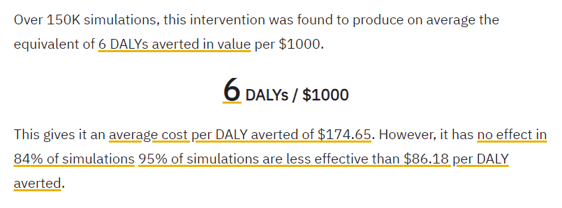
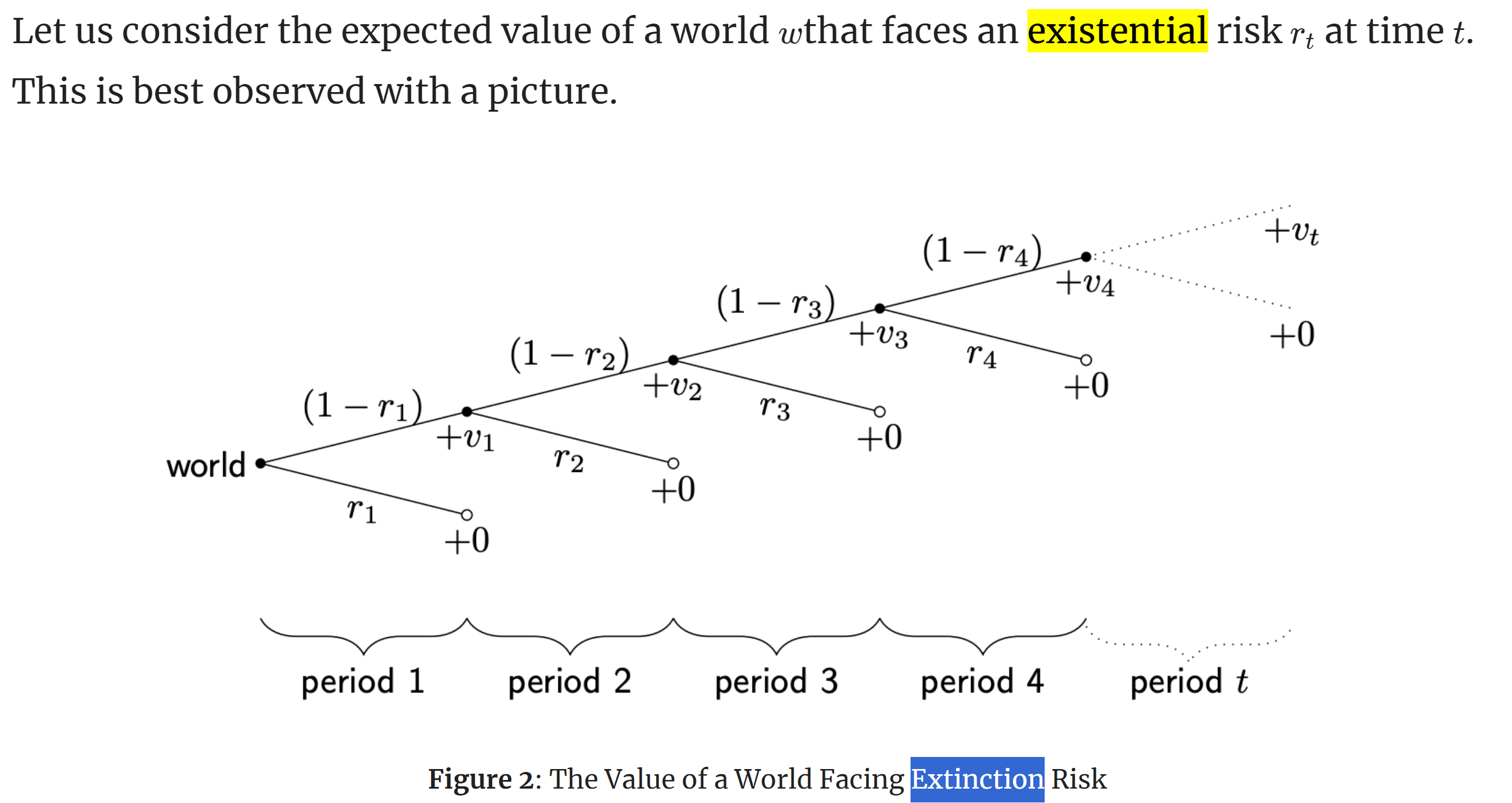


 Overview
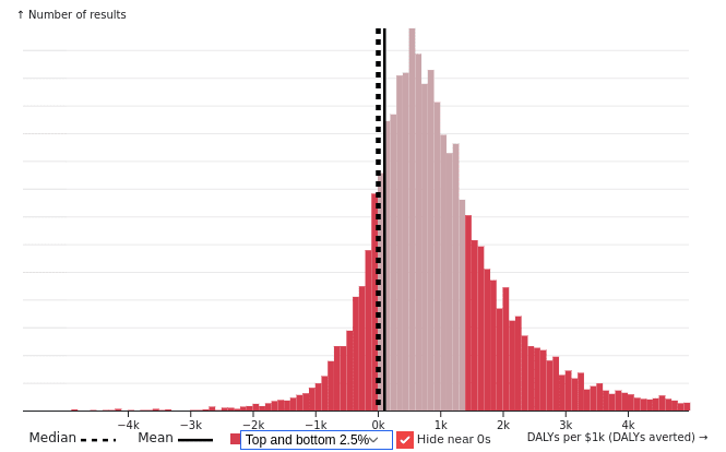
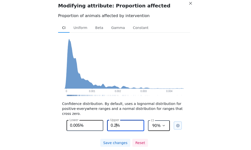
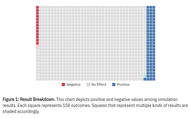
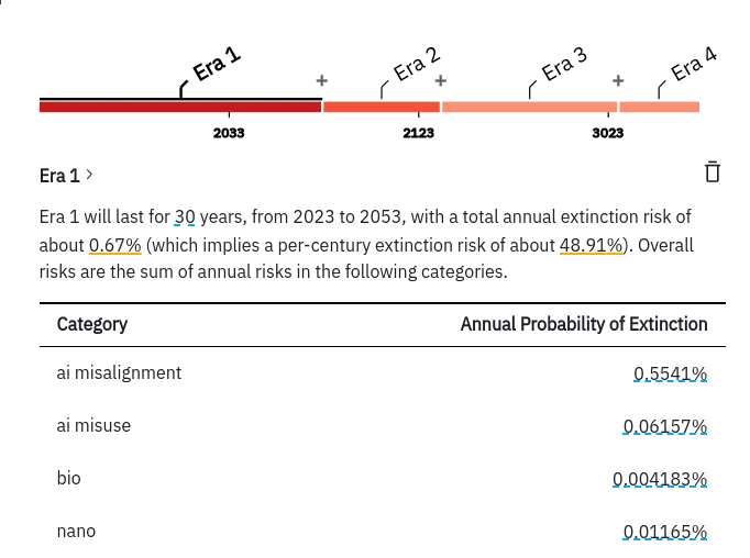

Excellent work. I've run out of good words to say about this Sequence. Hats off to the RP team.