A common first step towards incorporating uncertainty into a cost effectiveness analysis (CEA) is to express not just a point estimate (i.e., a single number) for an input to the CEA, but to provide some indicator of uncertainty around that estimate. This might be termed an optimistic vs. pessimistic scenario, or as the lower and upper bounds of some confidence or uncertainty interval. A CEA is then performed by combining all of the optimistic inputs to create an optimistic final output, and all of the pessimistic inputs to create a final pessimistic output. I refer to this as an ‘interval-based approach’. This can be contrasted with a fuller ‘probabilistic approach’, in which uncertainty is defined through the use of probabilistic distributions of values, which represent the range of possibilities we believe the different inputs can take. While many people know that a probabilistic approach circumvents shortcomings of an interval-based approach, they may not know where to even begin in terms of what different distributions are possible, or the kinds of values they denote.
I hope to address this in the current post and the accompanying application. Concretely, I aim to:
- Show how performing a CEA just using an interval-based approach can lead to a substantial overestimation of the uncertainty implied by one’s initial inputs, and how using a probabilistic approach can correct this while also enabling additional insights and assessments
- Introduce a new tool I have developed - called Distributr - that allows users to get more familiar and comfortable with a range of different distributions and the kinds of values they imply
- Use this tool to help generate a probabilistic approximation of the inputs GiveWell used in their assessment of Strongminds,[1] and perform a fuller probabilistic assessment based upon these inputs
- Show how this can be done without needing to code, using Distributr and a simple spreadsheet
I ultimately hope to help the reader to feel more capable and confident in the possibility of incorporating uncertainty into their own cost effectiveness analyses.
Propagating uncertainty and the value of moving beyond an interval-based approach
Cost effectiveness analysis involves coming up with a model of how various different factors come together to determine both how effective some intervention is, and the costs of its delivery. For example, when we think about distributing bed nets for malaria prevention, we might consider how the cost of delivery can vary across different regions, how the effects of bed net delivery will depend on the likelihood that people use the bed nets for their intended purpose, and the probability that recipients will install the bed nets properly. These and other factors all come together to produce an estimate of the cost effectiveness of an intervention, which will depend on the values we ascribe to the various inputs.
One way that a researcher might seek to express uncertainty in these inputs is by placing reasonable upper and lower bounds on their estimates for each of them. The researcher might then seek to propagate this uncertainty in the inputs into the anticipated uncertainty in the outputs by performing the same cost effectiveness calculations as they did on their point estimates on their upper bounds, and on their lower bounds, thereby producing corresponding upper and lower bounds on the final cost effectiveness.
An example of an interval-based approach is GiveWell’s assessment of Happier Lives Institute’s (HLI's) CEA for StrongMinds. The purpose of this post is not to provide an independent evaluation of Strongminds or HLI's assessment of it, nor is the key take away intended to be a critique of GiveWell having used an interval-based approach in that post.[2] Rather, I hope to guide the reader through an understanding of the limitations of this approach and then, using GiveWell’s numbers as a concrete starting point, show how a fuller probabilistic approach could be taken without reliance on advanced understanding of statistics or mathematics, nor a reliance upon coding.
The GiveWell post considers how various factors such as Social Desirability Bias among intervention recipients, Publication Bias in reports of mental health intervention effects, and Changing the Context in which the intervention is conducted might all impact what we should reasonably consider the efficacy of a mental health intervention such as Strongminds to be. These inputs are expressed in terms of a best guess, with a corresponding optimistic and pessimistic bound. These optimistic and pessimistic bounds are used to calculate optimistic and pessimistic estimates of the overall cost effectiveness of the intervention.
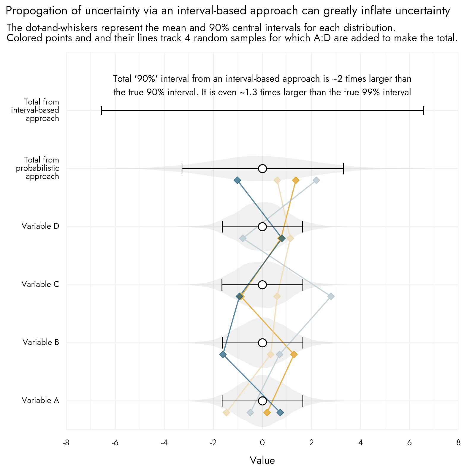
A key issue with propagating uncertainty in this way is that it can dramatically inflate the uncertainty of final outcomes that are calculated from the underlying input variables. We can see this by using a toy example, where a final total estimate is determined by the sum of four input variables - A, B, C, and D.
Let’s imagine that our uncertainty about the values of A, B, C, and D can be expressed as a classic bell curve distribution (i.e., a normal distribution) centered around 0, with a standard deviation of 1. This produces a mean of 0, and a 90% interval from approximately -1.6 to 1.6 for each input.[3] We’ll call these our pessimistic and optimistic bounds. Using an interval-based approach, we would produce a pessimistic and optimistic estimate for our total by summing each of these bounds. Our pessimistic and optimistic total values would then be roughly -6.4 and 6.4 respectively (-1.6 * 4, and 1.6 * 4).
In contrast, a probabilistic approach uses the whole distribution of each input: We generate the total estimate by taking samples from our A, B, C, and D distributions, each time adding these samples together to make the total. We then end up with a full distribution of total estimates, and can directly calculate the 90% interval for this distribution. Rather than going from roughly -6.4 to 6.4, the true 90% interval for the total goes from about -3.3 to 3.3.
This toy example is displayed in the plot below. When we properly calculate the numbers without rounding until the final summarization, we find that the 90% interval produced using an interval-based approach is twice as wide as that produced by the (accurate) probabilistic approach. It is even 1.3 times larger than the true 99% interval, clearly showing how the interval-based approach leads to very extreme estimates, substantially inflating our uncertainty. This represents something of a conservative example as to the possible levels of inflation that can be produced with an interval-based approach, because the inflation increases as we add more variables into the equation (many CEAs involve much more than 4 inputs), and can also vary depending on exactly how the variables are set to interact with one another (e.g. adding or multiplying), as well as on what distributions are used. For example, when multiplying together 4 values that are distributed log-normally, we observed that the interval-based approach generates a final estimate with bounds that are 13 times wider than the true level of uncertainty.
The reason we get this inflation is because, unless we have reasons to believe otherwise, we assume each of our input variables are independent of one another. When using an interval-based approach, however, it is as if we are saying not just that our input variables are all correlated with one another, but perfectly so: to make our final lower bound we take all 4 of the pessimistic inputs, and for our final upper bound, we take all 4 of the optimistic ones. In an example with just 4 normally distributed variables, the chance that we would draw 4 times in succession from at or above the central 90% of possible outcomes, all in the same positive or negative direction, is exceedingly small (5% * 5% * 5% * 5% = 0.000625%), and reflects an extreme and highly unlikely outcome. We’ve gone from pessimistic inputs to some of the most extremely bad outputs possible, and from optimistic inputs to the most fantastically good ones.
With reference to the example of bed nets for malaria above, it would be as if delivery is as expensive as in our highly pessimistic scenario, and the number of people using nets for fishing or some other purpose is as high as in our highly pessimistic scenario, and the proportion who install the nets properly is as low as our highly pessimistic scenario. Each of these might be a merely pessimistic outcome for each input, but it can be seen that when they all come together they create a very dire final outcome, and one which is exceedingly unlikely if each were already unlikely in isolation.
To avoid these pitfalls, we would ideally be able to more fully incorporate uncertainty into our assessments of cost effectiveness.
Tools and tips for generating distributions of uncertainty to use in CEAs
Existing tools for incorporating uncertainty
When seeking to utilize a probabilistic approach to uncertainty for a cost effectiveness analysis, one stumbling block may be a lack of familiarity with tools that can produce such distributions. We might stipulate that we think one of our inputs is normally distributed, but how do we get this distribution? Beyond directly using a programming language such as R or Python, a range of tools have been developed to help with generating and working with distributions.
Guesstimate allows the user to generate a host of probability distributions, which can also be connected together or passed through different functions to create CEAs built from a range of inputs and assumptions (for a brief tutorial, see here, and for a more detailed guide, here). Dagger is a similar tool geared towards modeling and quantifying uncertainty. Some tools more oriented towards business planning and project evaluation, such as Causal, also allow for the generation of models with uncertainty. Moving more towards coding-based approaches, the Quantified Uncertainty Research Institute has developed Squiggle, a programming language that is purpose built for working with uncertainty distributions (see here for a tutorial/explanation). Peter Wildeford of Rethink Priorities has implemented Squiggle as a Python programming language package SquigglePy. Several of these tools also have the nice feature that you don’t necessarily need to describe the statistical distribution in terms of its proper parameters, such as the mean and standard deviation, but can instead give a best guess and some bounds, and they will generate a corresponding distribution if possible. Finally, general purpose programming languages, notably R and Python, have access to essentially any distribution one can think of.
Introducing Distributr for exploring and generating probabilistic distributions
Beyond just knowing how to generate distributions, many people who might wish to incorporate uncertainty into their CEAs may simply be unfamiliar with or lack confidence in their knowledge of the range of different distributions available, and the kinds of values they imply. From discussions I’ve had with people thinking of incorporating uncertainty into CEAs (likewise for selecting priors in Bayesian analyses), lack of confidence in knowing what different distributions are possible and what they mean is more frequently mentioned than not knowing specific tools for generating them.
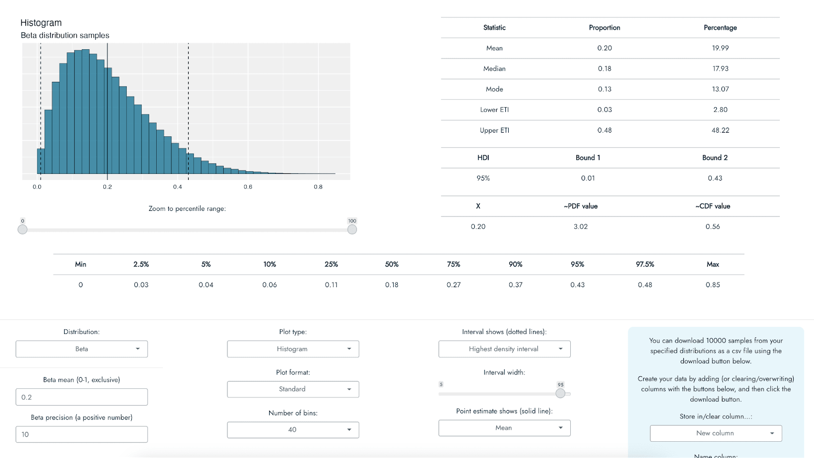
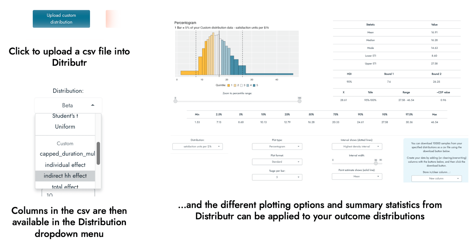
To help with my own understanding of different distributions, I have developed an application that can visualize a range of different probability distributions in multiple different ways, with a host of accompanying summary statistics (see the screenshot below). The app can be thought of as something like a distribution portfolio, in which you can explore and look at a range of different distributions on offer using different types of plot, along with several pieces of summary information, so as to better understand them and match them to your knowledge or expectations about a CEA input variable. The primary goal of the app was to help the user to become more familiar and confident in working with and understanding different distributions, but some of its functionality can be used to perform a probabilistic CEA.
The application - called Distributr - can be used here. Note that because this app runs on an R Shiny server, it is presently not well-suited for a high volume of users/requests, so if many people use it at once, it is possible that it will disconnect or time out.[4] It is also possible to download the code for the application from github, in which case you can run it directly on your own computer with R, without relying on the R Shiny server. A document outlining the different types of distributions, plots, and summary statistics available in the app can be found here (it is not necessary to read that documentation to continue with this post or to use the app).
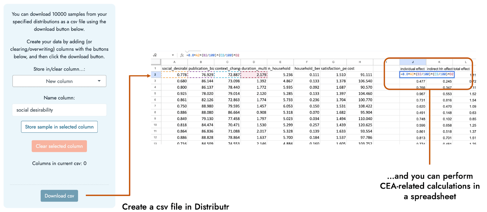
In addition to exploring what sorts of values are indicated by a range of distributions and their possible parameter specifications, Distributr also displays what command in R could be used to generate your own sample from the distribution, and also allows you to download a csv file including 10,000 samples from up to 10 different distributions in a single csv file. Hence, if you are not comfortable with programming, it would be possible to specify multiple distributions in the app, and then use Excel or Google Sheets to specify how these different distributions fit together to form a CEA based on the generated distributions.
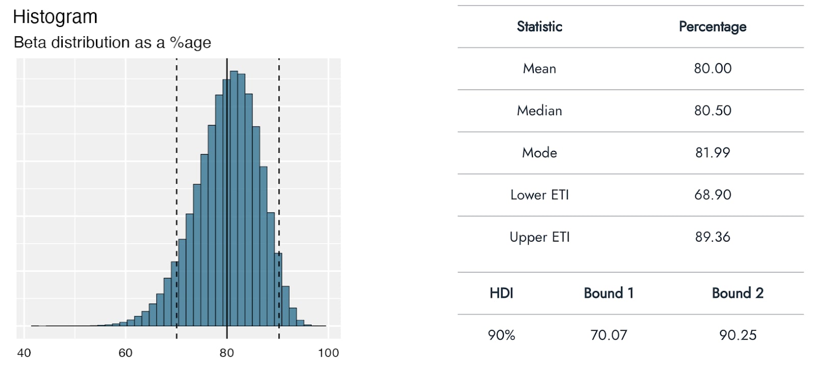
Using Distributr, I was able to visualize and assess the correspondence of a range of different distributions to the best, pessimistic, and optimistic guesses from GiveWell’s CEA of Strongminds. For example, GiveWell suggests a social desirability bias correction to the effect of the Strongminds intervention of approximately 80% [70%-90%]. I used a beta distribution to reflect this estimate being a proportion/percentage. Assuming that the pessimistic and optimistic ranges represent a 90% interval, this would correspond roughly to a beta distribution with a mean of .8 and precision of 40:
By using a range of distributions to make similar approximations to the estimates provided by GiveWell, it is possible to generate an entire set of probabilistic distributions corresponding to each of the input variables used in the Strongminds CEA. These can then be combined together to produce probabilistic estimates of cost effectiveness.
Approximating and running a probabilistic CEA for Strongminds based on GiveWell’s numbers
Approximating the GiveWell inputs
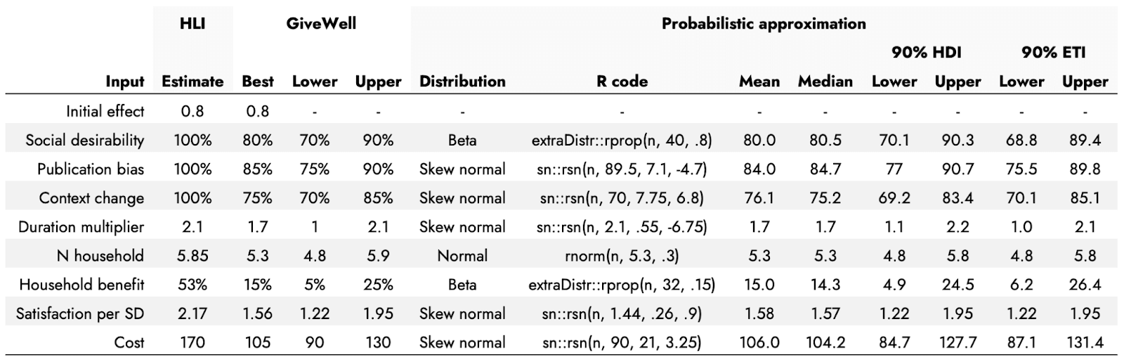
The table below shows HLI point estimates for different inputs to a CEA for Strongminds as reported in the GiveWell post, with additional inputs that GiveWell included in their CEA, along with GiveWell’s best, optimistic, and pessimistic estimates for these inputs. I include distributions that roughly correspond to these GiveWell estimates and an example piece of R code that would generate the respective distribution (in the Appendix, I show that similar conclusions to those below apply if just agnostic, uniform distributions are used instead).
I stress that these really are only approximate matches, and also that they are based on an assumption of the GiveWell estimates representing something like a mean for the best guess, and a 90% central interval for the optimistic and pessimistic bounds. These numbers would have to be changed if this were not the case, and in practice one would seek to generate these distributions in collaboration with the person proposing the plausible values, to ensure the distributions reflect the knowledge and expectations they are intended to encode. This process can also help to refine and become more explicit about one’s expectations. Some points to consider here would be not only what the uncertainty bounds represent, but also whether the point estimate reflects the mean, the median, the mode - which can diverge meaningfully when using distributions that are not symmetrical. As an example of where this kind of consultation would be useful, the Duration multiplier point estimate and bounds were particularly difficult to generate within a reasonable degree of similarity using a formal statistical distribution, and the generated values from the chosen distribution have a long tail that can skew into negative durations (which is not possible for this input). I therefore capped how low these values were allowed to go to 0.2 after sampling them from the distribution. A more appropriate distribution that would not need to be artificially capped, or a different cap, might be chosen after further discussion.[5]
The point of this procedure is therefore not to directly update the estimates provided by either GiveWell or by HLI, but to demonstrate - with a concrete and relevant example - how incorporating uncertainty might be done, and how such a probabilistic approach might plausibly lead to different conclusions and levels of uncertainty in the final estimates.
Performing the cost effectiveness calculations
In the CEA, we first need to calculate the expected effect for an individual directly undergoing the intervention. This is simply the product of Initial effect * Social desirability * Publication bias * Context change * Duration multiplier. Next, we can use this Individual effect estimate to calculate an expected Indirect household effect: how much those in the receiver’s household indirectly benefit from the receiver directly getting the intervention. This is the result of: Individual effect * Household benefit * (N household - 1). The Total effect of the intervention is then Individual effect + Indirect household effect.
Now that we have this estimated Total effect, we convert it to a general scale of ‘life satisfaction units’. This is done by getting the product of: Total effect * Satisfaction per SD. Next, we convert this to an estimate of how many of these ‘life satisfaction units’ we get per $1000 spent on the intervention: Total effect in satisfaction units * (1000 / Cost).
Finally, if we wish, we can compare this Life satisfaction units per $1k estimate with other interventions that have been estimated in terms of this same metric. In the GiveWell post, this is done relative to both GiveDirectly and the Against Malaria Foundation (AMF): Life satisfaction units per $1k Strongminds / Life satisfaction units per $1k of comparison intervention. HLI and GiveWell suggested that GiveDirectly achieved 8 Life satisfaction units per $1k, and AMF was given 81 on this metric by HLI, and 70 by GiveWell. We stick with the GiveWell estimate in our probabilistic analysis.
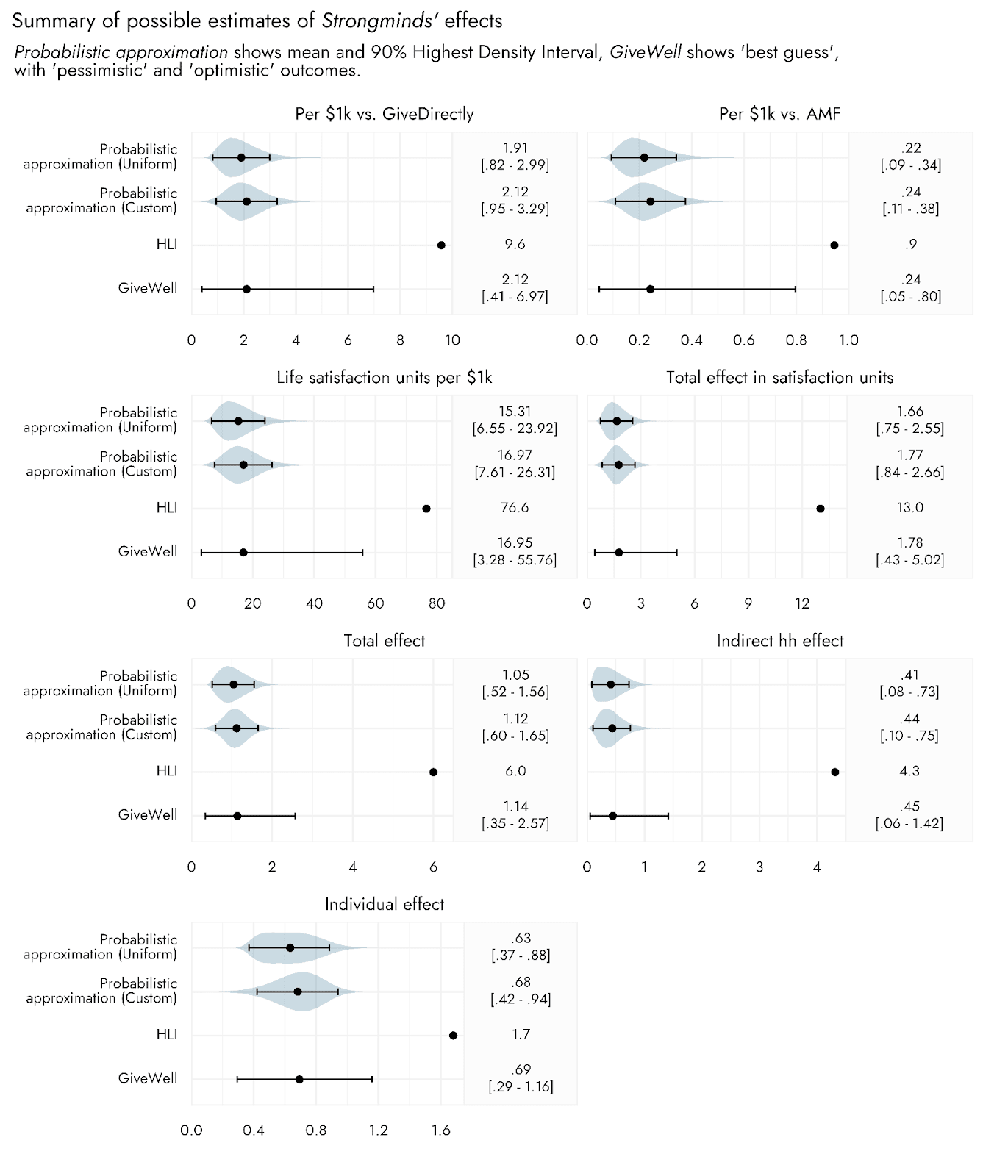
Now, we can see how these intermediate and final estimates compare when running a probabilistic approximation based on the optimistic and pessimistic scenarios of GiveWell, relative to using these scenario bounds as direct inputs in the above calculations.
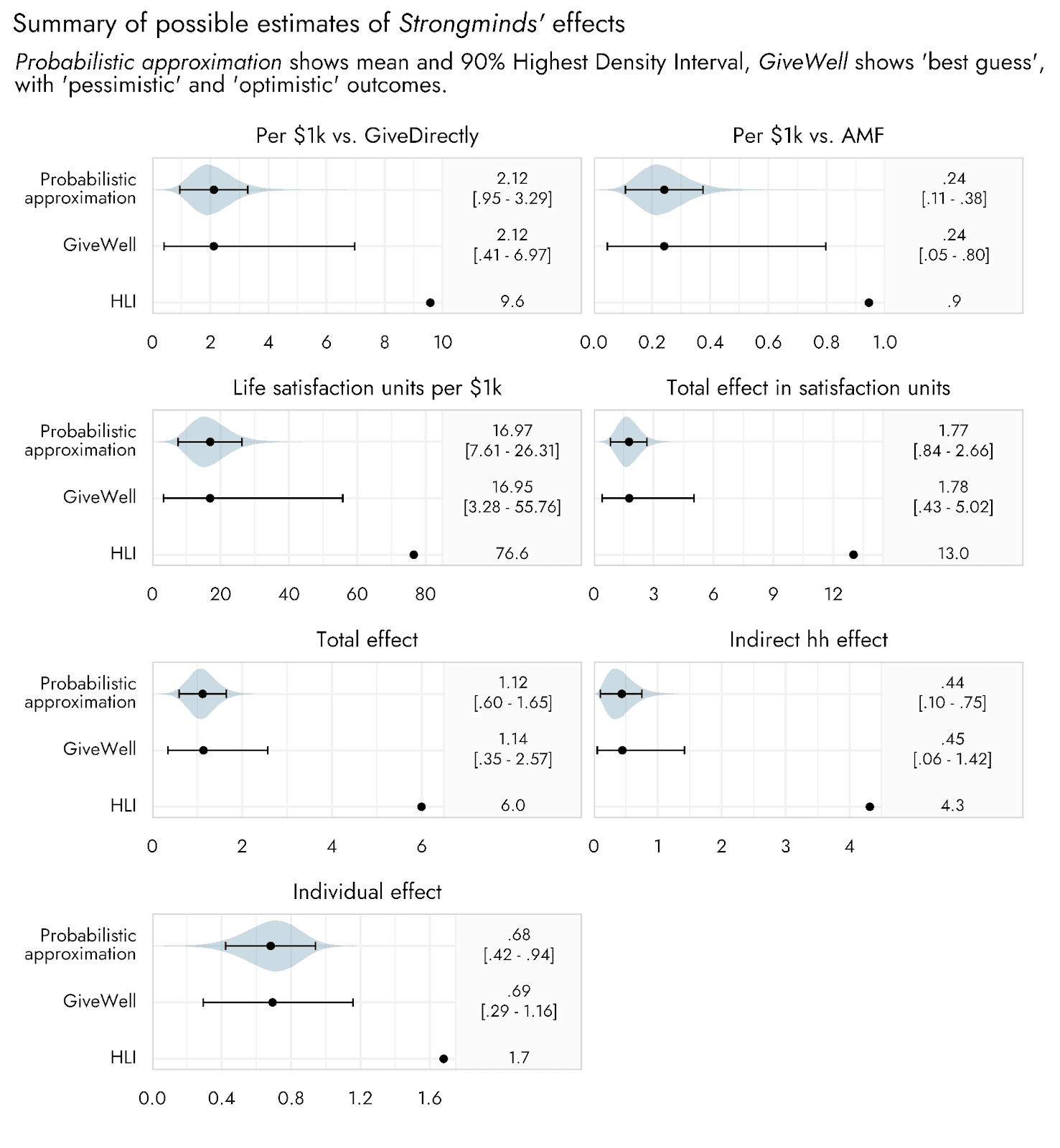
Moving from the initial stages of the CEA (the Individual effect) to the final stages (comparing life satisfaction units per $1000 relative to AMF or GiveDirectly), the width of the uncertainty bounds go from 1.7 times to 2.8 times larger for the estimates made via an interval-based approach relative to the probabilistic approximation. The upper estimates based upon a fuller probabilistic estimation of the effects of Strongminds are consequently much further from the HLI point estimates than are the upper bounds suggested in the GiveWell post.
Again, the extent of possible overestimation of uncertainty based upon using an interval-based approach would depend on exactly what those intervals represent, and would be different if taken to be something other than a 90% interval. This may even highlight a further limitation of the interval-based approach: we may not know exactly what the points and intervals are intended to represent. They could reflect the 90% or the 95% range of the data; one person’s understanding of ‘pessimistic’ may be very different from another’s. They could be the central 90% of values, cutting off the top and bottom 5%, or they could be the 90% most likely expected values. However, the only way this approach would not lead to at least some overestimation of uncertainty is if the bounds indicated the absolute maximum and minimum possible values for each input.
If the estimates from an interval-based approach show greater uncertainty than seems reasonable based upon a fuller probabilistic assessment, does this even matter? After all, the mean estimates come out effectively the same. It might even be argued that these wider uncertainty intervals are a good thing, perhaps representing a conservative or more humble reflection of our uncertainty.
I argue that it does matter - especially when it comes to assessing different programs relative to one another. We will discuss some approaches to comparing programs in the section Making probabilistic comparisons with other programs/interventions below, but put briefly, the probabilistic approach allows us to make much more nuanced assessments of programs. If we only have the intervals, then all we can reasonably say if an estimate for one program falls within the bounds of another is that we can neither confirm nor deny a difference between them. With a probabilistic approach, we can assess the relative likelihood of one program outperforming the other. Furthermore, with an interval-based approach, we have no idea how the plausibility of different values varies within that bounded region. Though it may seem conservative to err on the side of overstating our uncertainty, it risks being misleading in terms of dramatically overestimating the plausibility of extreme values.
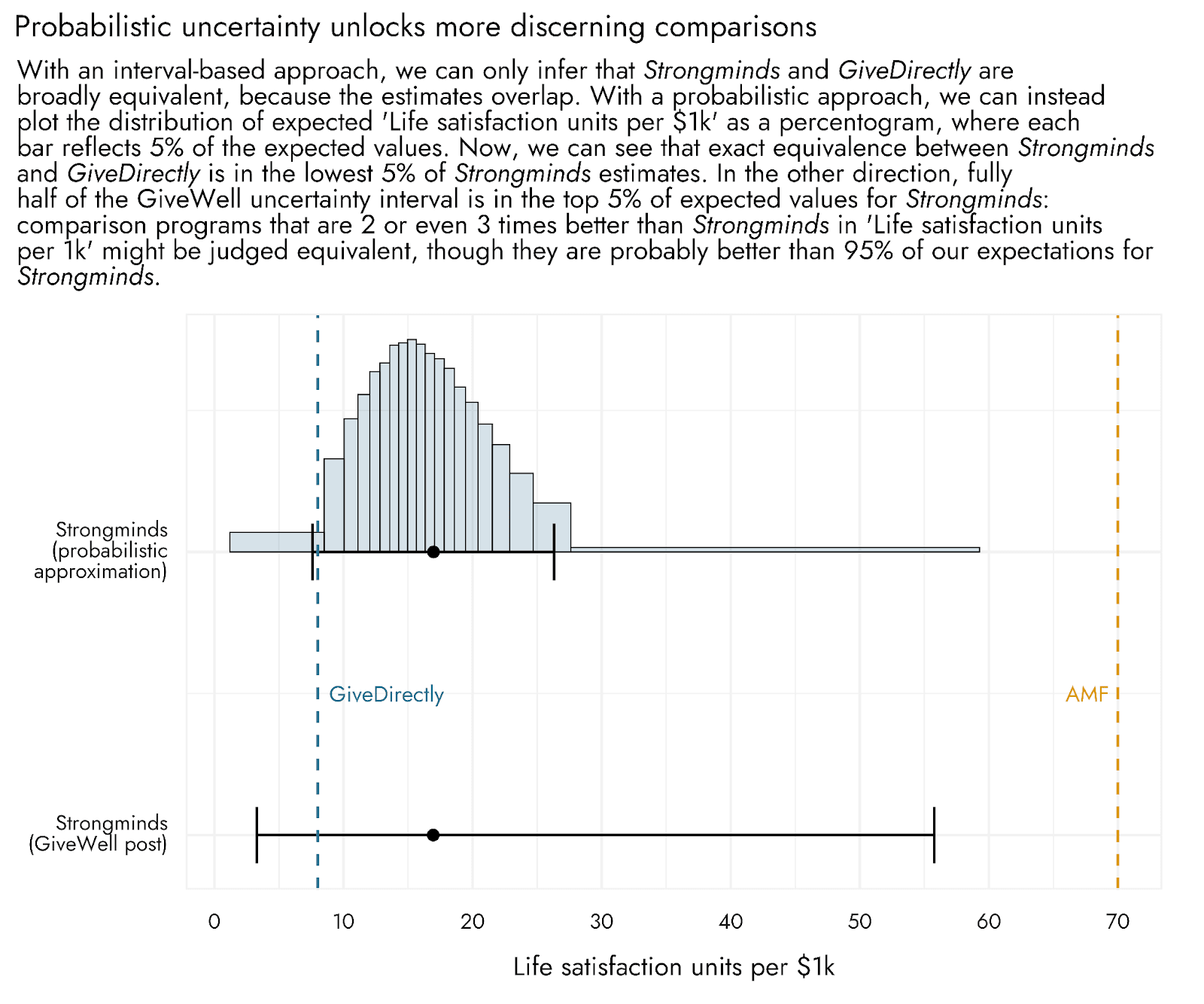
These points can be understood by looking at the plot below, which shows differences between the inferences that one might unlock when following a probabilistic approach, versus an interval-based approach, to comparisons amongst programs. Firstly, according to the probabilistic estimation, the chance that Strongminds is exactly equal to or worse than GiveDirectly seems quite low, representing the 5% most pessimistic of our potential outcomes (though it is certainly not out of the question). The uncertainty interval produced via the interval-based approach stretches considerably further out into more extremely negative outcomes for Strongminds, and may thus make these outcomes seem more plausible than they probably are.
In addition, and at the other extreme, a very large part of the GiveWell uncertainty interval - indeed the majority of it - covers the highest 5% of our probabilistic estimates for Strongminds. If we visually inspect the GiveWell pessimistic-optimistic range, we might conclude that it's reasonably likely that Strongminds produces ~30 life satisfaction units per $1k. After all, this value is much closer to the "best guess" than the "optimistic" value, and the interval provides no further information about how likely any given outcome is. However, if we consult the graph produced from the probabilistic approach, we can see that this outcome is in the most optimistic 5% of values and so is comparatively unlikely. The interval-based approach risks making such relatively extreme outcomes appear more likely than they actually are.
Indeed, using the interval-based approach, a comparison program might be two times better than 95% of our expectations for the program, but it would fall within the over-extended bounds produced by this approach, and could be considered as having little plausible difference in effectiveness. Note that the probabilistic approach does not outright reject the possibility of these values: we could directly calculate the chances we expect for values to appear across the whole range of plausible possibilities.
Using Distributr and a spreadsheet to do the calculations
The calculations and plots above were done in R, but it is also possible to use Distributr to generate a csv file of samples from the different inputs’ possible distributions. We can then just use Excel or Google sheets to perform calculations based on the samples, and summarize the resulting estimates, as was done in this sheet.[6] Hence, a large part of incorporating uncertainty into relatively simple CEAs such as this one could be done even if the user is most comfortable using spreadsheets as opposed to coding.
Visualizing CEA outcomes using Distributr
Having generated a set of outcome distributions, we are also not limited to using summary functions available in spreadsheet software. We can save the values of our estimates in a new csv file, and upload them to Distributr as custom distributions (the outcomes are available as a google sheet here). This allows us to fully visualize them and explore their implications using a host of different summary statistics available in Distributr.
Making probabilistic comparisons with other interventions
As well as providing bounds on estimates that more accurately reflect the propagation of uncertainty, using a probabilistic approach enables some additional types of comparisons and visualizations than would be possible if we used an interval-based approach.[7]
If we had a distribution of effectiveness estimates from a CEA for another project, we could directly compare the programs by subtracting one distribution from the other. The resulting distribution would reflect the distribution of uncertainty surrounding differences between the two assessed programs, and could also be summarized with a point estimate and different uncertainty intervals as desired, or via considering the relative probabilities of the range of plausible differences. This allows us to make much more fine-grained and sensitive comparisons than if we had to just judge whether or not the estimate for one program falls within the uncertainty bounds of another.
For comparisons with AMF and with GiveDirectly, we do not have a distribution of uncertainty, but we do have a point estimate (from GiveWell, as noted above, AMF appears to generate somewhere around 70 satisfaction units per $1k, and GiveDirectly around 8). We could calculate the proportion of our distribution of estimates for Strongminds that exceeds vs. falls below these comparison programs.
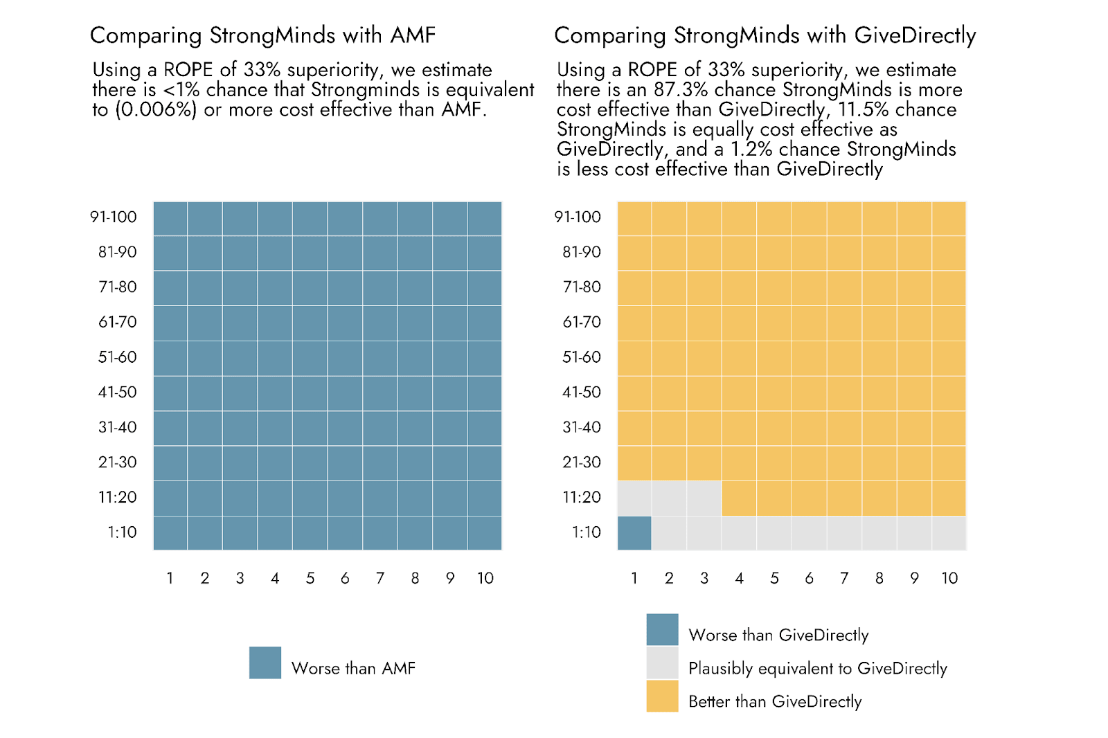
To convey that there is some uncertainty in the point estimates for AMF and GiveDirectly, or simply to reflect that we want to be somewhat conservative in deeming a new intervention clearly inferior or superior to an established comparison program, we could also add a range around these point estimates. Only if an estimate from our Strongminds distribution falls outside of this range might we suggest that the program appears to be better or worse. This is known as setting a Range of Practical Equivalence (ROPE). For the sake of demonstration, we set a ROPE around the estimates such that the compared interventions need to outperform one another by 33% in order to be deemed ‘different’ in their cost effectiveness.[8]
For visual clarity, and at the expense of some precision, we plot the outcomes of this procedure below as a pair of grid or ‘waffle’ plots. The totality of each grid represents 100% of the probabilistically estimated outcomes, and each square represents 1 percent of these outcomes. From these plots, Strongminds comes out looking pretty solid relative to GiveDirectly: The bulk of squares indicates superiority of Strongminds, and just a single square - representing 1.2% of the comparisons - indicates inferiority. However, for Strongminds vs. AMF, essentially the entirety of our probabilistic estimates favor AMF.
Summary and concluding remarks
As I hope to have demonstrated, incorporating uncertainty into CEAs using an interval-based approach can lead to substantial overestimates of the uncertainty in the final outputs. This issue can be rectified by making use of probabilistic distributions to represent that uncertainty.
Performing calculations for a CEA on random samples from these distributions more appropriately propagates uncertainty through the cost effectiveness model. In addition, having a full distribution of estimates opens up the possibility of different types of summary statistics (e.g., different point estimates, different ranges and types of interval), different ways of comparing one’s estimates to other programs, and ultimately different forms of visual presentation and inference.
There are numerous tools available for generating distributions of values for use in a CEA, from using a programming language such as R or Python, to using specialized software - much of which has been developed by people in or adjacent to the EA community for just this purpose. My goal in sharing Distributr was to make the exploration of different distributions easy for those without programming experience, as I think it is often lack of confidence or familiarity with different distributions that presents a bottleneck for people seeking to start adding uncertainty into their CEAs. However, Distributr can also be used to generate random samples from specified distributions and perform relatively simple probabilistic CEAs just with a spreadsheet, and then to visualize and explore the resulting distributions of outcomes.
Moving from an interval-based approach to a fuller probabilistic approach can substantially increase the validity and nuance of inferences, and even change the types of inference one can make. I hope this post, as well as the tools and code accompanying it, can make it easier to do so.
Acknowledgments

This post was written by Jamie Elsey with contributions from David Moss. Distributr was developed by Jamie Elsey. We would like to thank Ozzie Gooen for review of and suggestions to the final draft of this post.
Appendix
Uniform distributions also produce less extreme outcomes than those suggested by an interval-based approach
One particular worry may be that fitting these different distributions seems overly ambitious - we just can’t put distributions on our expectations like this, it implies too much certainty over the inputs. Although I would argue that we often do have quite specific expectations about what sort of distribution shapes are reasonable for our inputs, we don’t have to rely on a specific shape. The most agnostic type of distribution we can use is a uniform distribution, where all values within a set of bounds are equally plausible. Again, treating the specified intervals from the GiveWell post as a 90% interval, we can extend them 5% on either side to get a simple 100% interval, and generate uniform distributions within these bounds. This uniform distribution approach, while still making many fewer assumptions than our custom approach above, still suggests that the interval-based approach is generating inflated estimates.
- ^
This post is based upon an internal talk I gave to researchers at Rethink Priorities. The goal of the talk was to discuss ways of incorporating and visualizing uncertainty in cost effectiveness analyses (CEAs). In the days preceding the talk, GiveWell posted their assessment of Happier Lives Institute’s CEA for StrongMinds. That post provided a relevant and timely CEA that I could use as a concrete example for incorporating uncertainty, and is the example around which this post is oriented.
I use the GiveWell assessment of Strongminds as a springboard and concrete example, as I think this is much more interesting than working wholly in the abstract. I take the assessments from GiveWell as given for the purposes of demonstration, and did not conduct additional research to assess whether or not these estimates, or those of the Happier Lives Institute (HLI), are reasonable. I only engage with the numbers as presented in the aforementioned GiveWell post, not with the original HLI report or follow-up discussions from HLI and others. An original report from the Happier Lives Institute on the cost effectiveness of Strongminds can be found here, and a second report on household spillovers here. A response from HLI to the GiveWell post can be found here.
- ^
We are aware, for example, that several contributions, and indeed the winning contribution, to GiveWell’s ‘Change our minds’ contest focused on possible ways of incorporating uncertainty into GiveWell CEAs - see the list of entries here and a winning entry on uncertainty here.
The inclusion of only a point estimate for the 'HLI' numbers that follow should not be taken to reflect that HLI rely solely on point estimates in their evaluations either, rather it reflects the numbers presented in the GiveWell post. Some of estimates in HLI reports noted in footnote 1 do include intervals and probabilistic estimation, which we have not evaluated.
- ^
This simply means that 90% of the values generated from this distribution are expected to fall between -1.6 and 1.6, with 5% of values above and 5% of values below this interval.
- ^
I hope this doesn’t happen, but if when you reach this point you click that link and it just times out or doesn’t seem to work, this is the most likely reason, as the app does run properly live in a web browser when usage is not high.
- ^
In general, it is worth checking minimum and maximum generated values from input distributions to assess implausible or invalid values that might impact a CEA. I have also since added additional distributions to the app, such as the PERT distribution, which might be appropriate alternatives to the skew normal.
- ^
Note that given the more limited functionality of Google sheets relative to R, I summarized the estimates using a 90% central interval rather than a highest density interval, so the numbers are not exactly the same as in the plots (this can also be due to variation in the random sampling of the distributions, even if the same summary stats were used).
- ^
- ^
Note that this would equate to a ROPE on the comparison of A cost effectiveness / B cost effectiveness of about .75 to 1.33, not of .67 to 1.33: If A / B is 1.33, then A is 1.33 times better than B. If A / B is .75, then B is 1.33 times better than A. The magnitude of this ROPE is completely arbitrary and chosen just for the purposes of demonstration, but in concrete scenarios decision-makers may have various practical reasons to be interested in whether an intervention is more than x times better than another.
Thanks a lot for this post, it definitely helped me clarify my thinking around modeling uncertainty. Excited to explore some of the tools you mentioned!
Executive summary: A cost effectiveness analysis using interval estimates for inputs can greatly overestimate uncertainty. Modeling inputs with probability distributions instead leads to more accurate uncertainty estimates and enables additional types of inference.
Key points:
This comment was auto-generated by the EA Forum Team. Feel free to point out issues with this summary by replying to the comment, and contact us if you have feedback.
I don't know if this is useful to you, but we have a somewhat easier way of solving the same problem using what we call a simplified Monte Carlo estimation technique. This is described in the following post:
https://forum.effectivealtruism.org/posts/icxnuEHTXrPapHBQg/a-simplified-cost-effectiveness-estimation-methodology-for
It is not quite as accurate as your method because it approximates the probability distributions as a three-value distribution, but it addresses the issue of CEA inputs being uncorrelated and can be done in any spreadsheet without a need of using any extra tools or web services. You just calculate for all combinations of inputs, and then use standard spreadsheet tools like cumulative probability plots or histogram calculators to get the probability distribution of results:
Thanks for your comment @Robert Van Buskirk, and great that you are also thinking of ways to incorporate uncertainty into CEAs. You note that your way also solves 'the same problem', but a key aspect of what we are arguing (and what others have suggested) is not just that a proper monte carlo approach avoids objective issues with an interval-based approach, but that it provides a wealth of more nuanced information and allows for much more discerning assessments to be made. This is approximated by the approach you suggest, but not fully realised. For example ‘A histogram of the full set of CE results is then constructed to illustrate the full range of possible CE values’ - but by definition the histogram won’t include the full range of possible values because values beyond the average of the top and bottom thirds are not included in the calculations. This might obscure or underestimate the possibility of extreme outcomes.
My second concern would just be that if one has the capacity to define what the average of the bottom third of the expected values are, and the average of the top third, this is in all likelihood enough information for defining an approximate distribution, or one could simply select a uniform distribution. In that case, why not just do a proper monte carlo? The main answer to this is often just that people don’t have the confidence to consider a possible probability distribution that might work, and that was the key thing I’m trying to help with in developing and sharing this application
Thanks Jamie: our method is most useful when one has a relatively small sample of field data. In that case it is easy to calculate the averages of the bottom third, middle third, and top third of values and this is good enough because the data sample is not sufficient to specify the distribution with any greater precision.
Our method can also be calculated in any spreadsheet extremely easily and quickly without using any plug-ins or tools.
But agreed, if someone has the time, data and capacity, your method is better.
Thanks for sharing! Monte Carlo simulations are useful to work with distributions of different types, but I also wanted to note there are some nice results one can use when working with just lognormals or normals. If for nothing else, these may be useful for Fermi estimates.
Uncertainty of the product between independent lognormal distributions without Monte Carlos
If Y is the product of independent lognormal distributions X_1, X_2, ..., and X_N, and r_i is the ratio between the values of 2 quantiles of X_i (e.g. r_i = "95th percentile of X_i"/"5th percentile of X_i"), I think the ratio R between the 2 same quantiles of Y (e.g. R = "95th percentile of Y"/"5th percentile of Y") is e^((ln(r_1)^2 + ... + ln(r_N)^2)^0.5)[1]. For the particular case where all input distributions have the same uncertainty, r_i = r, and therefore R = r^(N^0.5). This illustrates your point that performing point estimates with pessimistic and optimistic values overestimates uncertainty:
The naive approach would only make sense if the input distribution were perfectly (or very highly) correlated.
Sum and product of independent normal distributions without Monte Carlos
If X_1, X_2, ..., and X_N are independent normal distributions, and Y = X_1 + X_2 + ... + X_N:
If X_1, X_2, ..., and X_N are independent normal distributions, and Y = X_1 X_2 ... X_N:
After getting the mean and variance of Y, one could obtain e.g. its 5th percentile in google sheets using NORMINV(0.05, E(Y), V(Y)^0.5).
Product of independent lognormal distributions without Monte Carlos
If X_1, X_2, ..., and X_N are independent lognormal distributions, and Y = X_1 X_2 ... X_N, ln(Y) = ln(X_1) + ln(X_2) + ... + ln(X_N), so:
One would obtain E(ln(X_i)) and V(ln(X_i)) in the same way one would get the mean and variance of a normal distribution given 2 points, but using their logarithms. If a_i and b_i are 2 values of X_i such that P(X_i <= a_i) = P(X_i >= b_i) (for example, a_i and b_i could be the 5th and 95th percentile, 10th and 90th percentile, 25th and 75th percentile, etc.):
After getting the mean and variance of ln(Y), one could obtain e.g. the 5th percentile of Y in google sheets using EXP(NORMINV(0.05, E(ln(Y)), V(ln(Y))^0.5)).
I used this formula here.