Suppose I have several point-estimates for the fuel efficiency of my car - I can easily take a weighted average of these to make an aggregate point estimate, but it’s not clear how I could turn them into an interval estimate without a heavy dose of personal bias.
You could create a mixture distribution, you could fit a lognormal whose x% confidence interval is the range expressed by the points you've already found, you could use your subjective judgment to come up with a distribution which could fit it, you could use kernel density estimation (https://en.wikipedia.org/wiki/Kernel_density_estimation).
In your number of habitable planets estimate, you have a planetsPerHabitablePlanet estimate. This is an interesting decomposition. I would have looked at the fraction of planets which are habitable, and probably fit a beta distribution to it, given that we know that the fraction is between 0 and 1. This seems a bit like a matter of personal taste, though.
I agree with your claim that lognormal distributions are a better choice than normal. However this doesn't explain whether another distribution might be better (especially in cases where data is scarce, such as the number of inhabitable planets).
For example, the power law distribution has some theoretical arguments in its favour and also has a significantly higher kurtosis, meaning there is a much fatter tail.
Related to which type of distribution is better, in this episode of The 80,000 Hours Podcast (search for "So you mentioned, kind of, the fat tail-ness of the distribution."), David Roodman suggests using the generalised Pareto distribution (GPD) to model the right tail (which often drives the expected value). David mentions the right tails of normal, lognormal and power law distributions are particular cases of the GDP:
Robert Wiblin: This kind of log-normal or normal curve, or power law, are they all special cases of this generalized family [GPD]?
David Roodman: Their tails are.
So, fitting the right-tail empirical data to a GPD is arguably better than assuming (or fitting the data to) one particular type of distribution:
[David Roodman:]
So what you can do is you can take a data set like, all geomagnetic disturbances since 1957, and then look at the [inaudible 00:59:09] say, 300 biggest ones. What’s the right tail of the distribution? And then ask which member of the generalized Pareto family fits that data the best? And then once you’ve got a curve that you know … you know for theoretical reasons is a good choice, you can extrapolate it farther to the right and say, “What’s a million year storm look like?”
And one also has to be careful about out of sample extrapolations. But I think it’s more grounded in theory, this is, to use the generalized Pareto family, because it is analogous to using the normal family when constructing usual standard errors. Than, to, for example, assume that geomagnetic storms follow a power law, which was done in one of the papers that reached the popular press. So there was a Washington Post story some years ago that said the chance of a Carrington-size storm was like 12% per decade. But that was assuming a power law, which has a very fat tail. When I looked at the data, I just felt that that … and allowed the data to choose within a larger and theoretically motivated family. It did not, the model fit did not gravitate towards the power law.
Cool. To be clear, I think if anyone was reading your piece with any level of care or attention, it would be clear that you were comparing normal and lognormal, and not making any stronger claims than that.
Point estimates are fine for multiplication, lossy for division
I think one caveat here is that, if we want to obtain an expected value as output, the input point estimates should refer to the mean instead of the median. They are the same or similar for non-heavy-tailed distributions (like uniform or normal), but could differ a lot for heavy-tailed ones (like exponential or lognormal). When setting a lognormal to a point estimate, I think people often use the geometric mean between 2 percentiles (e.g. 5th and 95th percentiles), which corresponds to the median, not mean. Using the median in this case will underestimate the expected value, because it equals (see here):
E(X) = Median(X)*e^(sigma^2/2), where sigma^2 is the variance of log(X).
Here you mention that this "lognormal mean" can lead to extreme results, but I think that is a feature as long as we think the lognormal is modelling the right tail correctly. If we do not think so, we can still use the mean of:
Truncated lognormal distribution.
Minimum between a lognormal distribution and a maximum value (after which we think the lognormal no longer models the right tail well).
Interval estimates are prone to personal bias. It’s easy to create an interval estimate intuitively. When objectivity is important and the evidence base is sparse, point estimates are easier to form and are more transparent.
In my mind:
Being objective is about faithfully representing the information we have about reality, even if that means being more uncertain.
The evidence base being sparse suggests we are uncertain about what reality actually looks like, which means a faithful representation of it will more easily be achieved by intervals, not point estimates. For example, I think using interval estimates in the Drake equation in much more important that in the cost-effectiveness analyses of GiveWell's top charities.
One compromise to achieve transparency while mainting the benefits of interval estimates is using pessimistic, realistic and optimistic point estimates. One the one hand, this may result in wider intervals because the product between 2 5th percentiles is rarer than a 5th percentile, so the pessimistic final estimate will be more pessimistic than its inputs. On the other hand, we can think as the wider intervals as accounting for structural uncertainty of the model.
Thanks for your feedback, Vasco. It's led me to make extensive changes to the post:
More analysis on the pros/cons of modelling with distributions. I argue that sometimes it's good that the crudeness of point-estimate work reflects the crudeness of the evidence available. Interval-estimate work is more honest about uncertainty, but runs the risk of encouraging overconfidence in the final distribution.
I include the lognormal mean in my analysis of means. You have convinced me that the sensitivity of lognormal means to heavy right tails is a strength, not a weakness! But the lognormal mean appears to be sensitive to the size of the confidence interval you use to calculate it - which means subjective methods are required to pick the size, introducing bias.
Overall I agree that interval estimation is better suited to the Drake equation than to GiveWell CEAs. But I'd summarise my reasons as follows:
The Drake Equation really seeks to ask "how likely is it that we have intelligent alien neighbours?", but point-estimate methods answer the question "what is the expected number of intelligent alien neighbours?". With such high variability the expected number is virtually useless, but the distribution of this number allows us to estimate the number of alien neighbours. GiveWell CEAs probably have much less variation and hence a point-estimate answer is relatively more useful
Reliable research on the numbers that go into the Drake equation often doesn't exist, so it's not too bad to "make up" interval estimates to go into it. We know much more about the charities GiveWell studies, so made-up distributions (even those informed by reliable point-estimates) are much less permissible.
You have convinced me that the sensitivity of lognormal means to heavy right tails is a strength, not a weakness!
Yes, but only as long as we think the heavy right tail is being accurately modelled! Jaime Sevilla has this post on which methods to use to aggregate forecasts.
Interval-estimate work is more honest about uncertainty, but runs the risk of encouraging overconfidence in the final distribution.
I think it is worth flagging that risk, but I would say:
In general, if a given method is more accurate, it seems reasonable to follow that method everything else equal.
One can always warn about not overweighting results estimated with intervals.
Intuitively, there seems to be much higher risk of being overconfident about a point estimate than about a mean estimated with intervals together with a confidence interval. For example, regarding Toby Ord's best guess given in Table 6.1 of The Precipice for the existential risk from nuclear war between 2021 and 2120, I think it is easier to be overconfident about A than B:
A. 0.1 %.
B. 0.1 % (90 % confidence interval, 0.03 % to 0.3 %). Toby mentions that:
"There is significant uncertainty remaining in these estimates and they should be treated as representing the right order of magnitude—each could easily be a factor of 3 higher or lower".
But the lognormal mean appears to be sensitive to the size of the confidence interval you use to calculate it - which means subjective methods are required to pick the size, introducing bias.
Yes, for the same median, the wider the interval, the greater the mean. If one is having a hard time linking 2 given estimates to a confidence interval, one can try the narrowest and widest reasonable intervals, and see if the lognormal mean will vary a lot.
We know much more about the charities GiveWell studies, so made-up distributions (even those informed by reliable point-estimates) are much less permissible.
I think people with knowledge about GiveWell's cost-effectiveness analyses would be able to come up with reasonable distributions. A point estimate is equivalent to assigning probability 1 to that estimate, and 0 to all other outcomes, so it is easy to come up with something better (although it may well not be worth the effort).
I think I have been trying to portray the point-estimate/interval-estimate trade-off as a difficult decision, but probably interval estimates are the obvious choice in most cases.
So I've re-done the "Should we always use interval estimates?" section to be less about pros/cons and more about exploring the importance of communicating uncertainty in your results. I have used the Ord example you mentioned.
Point estimates are fine for multiplication, lossy for division
One way of getting around this is transforming all divisions into multiplications. For example, one can calculate E(X/Y) from E(X)*E(1/Y) (assuming independence), instead of using E(X)/E(Y). Computing E(1/Y) will require using Guesstimate or similar, but then the mean can be used in a spreadsheet without having to run a full Monte Carlo simulation, which would take longer.
I am not sure, but I think a similar approach can be followed for most estimates. For example, one can use Guesstimate to obtain E(X^alpha) or E(log(X)), instead of using E(X)^alpha or log(E(X)).
Using intervals is still useful to get ranges for the outputs in a principled way, but I wonder whether the expected value alone is enough. I think expected utility is all that matters, so there is a sense in which the expected value captures all the relevant information.
I suppose I have been using interval estimates because I think they can inform how much the expected value might change in response to new information, which is useful to know. However, I am not confident uncertainty, which is what can be directly observed from the outputted intervals, is a good proxy for resilience.
I think I have come to believe assessing resilience doing a sensitivity analysis with point estimates derived from distributions is usually better than trying to evaluate it based on the uncertainty of the final result.
Note that 1/Y is generally not well defined when Y's range contains 0, and it's messy when it approaches it, and when both X and Y contains both positive and negative parts. My preferred solution is to either look at Xs and Ys that are both positive, or to look at the joint pdf of X and Y, rather than the sum.
Note that 1/Y is generally not well defined when Y's range contains 0, and it's messy when it approaches it
I agree. Just one note, I think a distribution for Y which encompasses 0 cannot be correct, because it would lead to infinities, which I am happy to reject. Can you give some examples in which Y (i.e. a distribution in the denominator) is defined such that it could not be zero, but you still found messiness?
when both X and Y contains both positive and negative parts
For this case, one can get point estimates from:
E(X) = P(X > 0)*E(X | X > 0) + P(X < 0)*E(X | X < 0).
E(1/Y) = P(Y > 0)*E(1/Y | Y > 0) + P(Y < 0)*E(1/Y | Y < 0).
I think that in practice you (almost) always want to calculate lives/$, not $/life
Yes, I prefer to calculate the cost-effectiveness in terms of benefits per unit cost. This way, the expected cost-effectiveness can be multiplied by the cost to obtain the expected benefits. In contrast, the cost cannot be divided by the expected cost per unit benefit to obtain the expected benefits.
Another advantage of benefits per unit cost is that they always increase with the goodness of the intervention, whereas the cost per unit benefit has a more confusing relationship (when it can be both positive and negative).
the cost is practically never zero
Yes, I do not think the cost can be zero. Even if the monetary cost is zero, there are always time costs.
This is a crosspost from the new Animal Welfare Alignment Newsletter by Anima International. You can subscribe on Substack if you are interested in following these efforts. Audio reading also available on Substack.
The goals of this post are to:
1. Raise a question I see as crucially important to the goal of aligning AI to animal welfare...
Hello! I'm Justin Portela. I got hired by GWWC to make YouTube videos after AI in Context did such a kickass job.
My channel is using that same cinematic, high-production value beauty to talk about everything in the EA universe that isn't AI.
...
This is a linkpost for Request for Proposals: Research and Applied Work on Digital Minds.
I'm glad to announce a request for proposals for research and applied work on digital minds at Longview Ph...
I explore the pros and cons of different approaches to estimation. In general I find that:
interval estimates are stronger than point estimates
the lognormal distribution is better for modelling unknowns than the normal distribution
the "lognormal" mean is better than the arithmetic mean for building aggregate estimates
These differences are only significant in situations of high uncertainty, characterised by a high ratio between confidence interval bounds. Otherwise, simpler approaches like point estimates & the arithmetic mean are fine.
Summary
I am chiefly interested in how we can make better estimates from very limited evidence. Estimation strategies are key to sanity-checks, cost-effectiveness analyses and forecasting.
Speed and accuracy are important considerations when estimating, but so is legibility; we want our work to be easy to understand. This post explores which approaches are more accurate and when the increase in accuracy justifies the increase in complexity.
My key findings are:
Interval (or distribution) estimates are more accurate than point estimates because they capture more information. When dividing by an unknown of high variability (high ratio between confidence interval bounds) point estimates are significantly worse.
It is typically better to model distributions as lognormal rather than normal. Both are similar in situations with low variability, but lognormal appears to better describe situations of high variability.
The "lognormal" mean is good for building aggregate estimates. By calculating the mean of a lognormal distribution for which our inputs form a confidence interval, we capture the positive skew typical of more variable distributions.
In general, simple methods are fine while you are estimating quantities with low variability. The increased complexity of modelling distributions and using geometric means is worthwhile when the unknown values are highly variable.
Interval vs point estimates
In this section we will find that for calculations involving division, interval estimates are more accurate than point estimates. The difference is most stark in situations of high uncertainty.
Interval estimates, for which we give an interval within which we estimate the unknown value lies, capture more information than a point estimate (which is simply what we estimate the value to be). Interval estimates often include the probability that the value lies within our interval (confidence intervals) and sometimes specify the shape of the underlying distribution. In this post I treat interval estimates as distribution estimates as the same thing.
Here I attempt to answer the following question: how much more accurate are interval estimates and when is the increased complexity worthwhile?
Core examples
I will explore this through two examples which I will return to later in the post.
Fuel Cost: The amount I will spend on fuel on my road trip in Florida next month. The abundance of information I have about fuel prices, the efficiency of my car and the length of my trip means I can use narrow confidence intervals to build an estimate.
Inhabitable Planets: The number of planets in our galaxy with conditions that could harbour intelligent life. The lack of available information means I will use very wide confidence intervals.
Point estimates are fine for multiplication, lossy for division
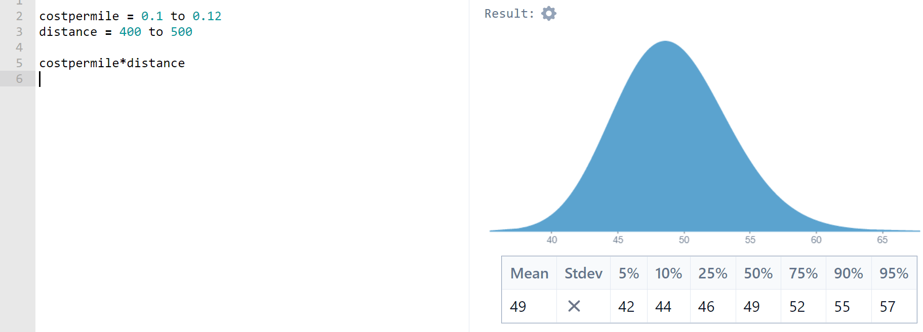
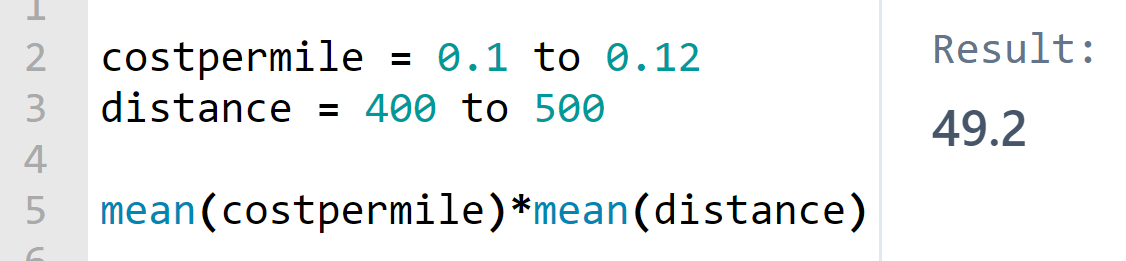
Let’s start with Fuel Cost. Using Squiggle (which uses lognormal distributions by default: see the next section for more on why), I enter 90% confidence intervals to build distributions for fuel cost per mile (USD per mile) and distance of my trip (miles). This gives me an expected fuel cost of 49.18USD
What if I had used point estimates? I can check this by performing the same calculation using the expected values of each of the distributions formed by my interval estimates.
I get the same answer. In fact, this applies in all cases: if X and Y are normally or lognormally distributed,
E(X)E(Y)=E(XY)
In other words, the mean of the product of two normal/lognormal distributions is the product of their means. The only drawback of using point-estimates for multiplication is that you only get a numerical answer - you lose the shape of the distribution.
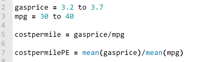
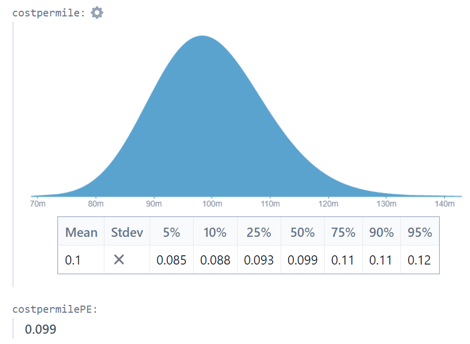
What about division? Put simply,
E(1/Y)≠1/E(Y)
so
E(X/Y)≠E(X)/E(Y)
Division will be lossy when you use point estimates. But how bad is it?
Using the Fuel Cost example we find that the point estimate result (0.099048) is within 1% of the interval estimate result (0.099809).
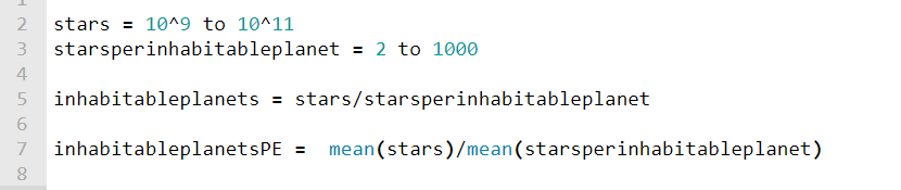
Now let’s turn to the inhabitable planets example. I use interval estimates for the number of stars in the galaxy and the number of stars per inhabitable planet. Because of the uncertainty the bounds of my intervals differ by 2-3 orders of magnitude.
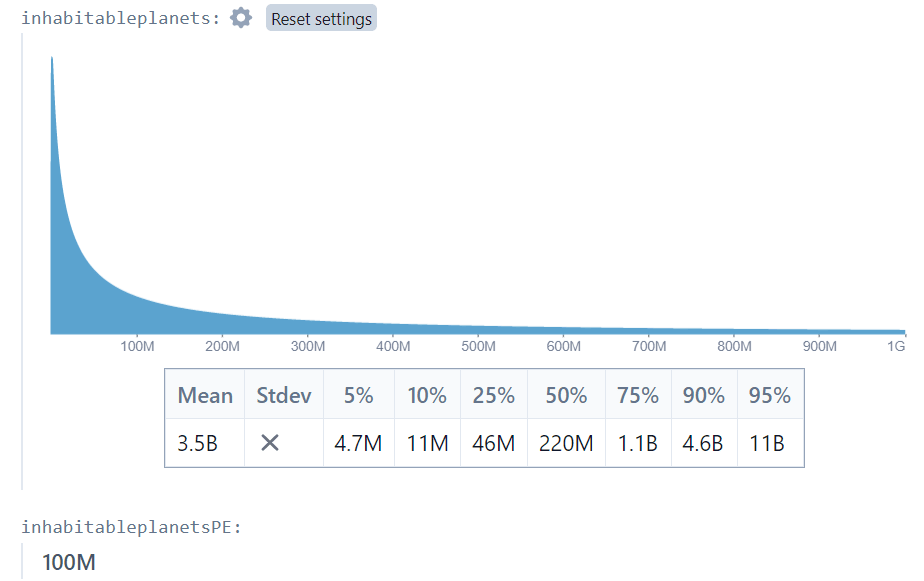
I find that the interval-estimate approach gives an expected number of inhabitable planets of 3.5 billion, while my point-estimate approximation is just 100 million! Clearly when there are very high levels of uncertainty, dividing by a point estimate is inaccurate. Not only that, but the point estimate answer provides no information on the shape of the possible outcomes. The interval estimate approach shows us that although the expected number of planets is 3.5 billion, the median is just 220 million.
This heavy-tailed behaviour helps explain where the Drake Equation (which relies upon point-estimates of highly uncertain values and suggests that we should have heard from aliens by now) goes wrong: using interval estimates we can show that although the expected number of interstellar alien neighbours is high, the median is much lower. My very rough attempt finds a mean of 4700 alien neighbours, with a a 25-50% chance of none at all (although I may be pushing Squiggle past its limits).
Should we always use interval estimates?
Using interval estimates as inputs
As we have seen, interval estimates are better for modelling uncertainty. They do not introduce mathematical error and they can store more information about what we know.
In a sense a point estimate is a distribution estimate: one that assigns probability 1 to the point estimate and 0 to everything else. This means it isn't hard to improve upon. However, if we don't have strong objective evidence for the shape of the distribution, we have to use personal judgement to estimate it. If transparency and impartiality are important, this can be a problem.
Suppose I do a quick google search and determine that the fuel efficiency of my car is supposed to be 47mpg. If I'm estimating the fuel cost for an expense form, using this value makes sense: the person reading the form can verify that this is an objective estimate of my car's efficiency. If I am doing he calculation for myself, on the other hand, it might make sense to use an interval estimate using my personal judgement (something like a 90% C.I. of 40 to 47mpg, on the basis that my car is no longer new and that cars don't achieve their theoretical efficiency in real-world conditions).
Using interval estimates as outputs
When constructing an estimate from multiple sub-estimates, as I would in the Fuel Cost and Inhabited Planets examples, a key challenge is communicating the level of uncertainty in the final result.
On their own, point-estimates do not communicate any nuance. They should be paired with a statement on the uncertainty of the result, like "this value is highly uncertain and could be off by an order of magnitude".
The trouble is that it's difficult to know just how uncertain the final result is. Even when we calculate using interval estimates, the reliability of the final distribution is highly uncertain. Look back at the Inhabited Planets example in the previous section: we find a 90% confidence interval of 4.7 million to 11 billion inhabitable planets in our galaxy. But this only gives a flavour of the likely distribution of inhabited planets. The 90% confidence interval, calculated from two rough sub-estimates, just isn't trustworthy.
So even though interval outputs communicate that the value is uncertain, readers may still overestimate the reliability of the estimate.
Toby Ord gives a good example of how to convey uncertainty in the Precipice. He accompanies table 6.1, which provides point-estimates for the magnitudes of various existential risks over the next 100 years, with the qualifier:
There is significant uncertainty remaining in these estimates and they should be treated as representing the right order of magnitude - each could easily be a factor of 3 higher or lower.
It's nice because the description of the uncertainty is itself imprecise, which dissuades us from being over-confident in it.
[Thanks to Vasco Grilo for highlighting this example]
General findings: interval vs point estimates
I did some more experimentation on Squiggle to generalise the findings slightly.
It's OK to multiply point-estimates. They will give the same mean as the mean of the product of two distributions.
Dividing by a point-estimate is accurate when the ratio between the interval bounds is low, and performs poorly when the ratio is more than 2. For example:
When dividing by a (lognormal, 90% C.I.) distribution where the upper bounds are 1.2 times the lower bounds, the point-estimate approach underestimates by 0.3%
When dividing by a (lognormal, 90% C.I.) distribution where the upper bounds are 2 times the lower bounds, the point-estimate approach underestimates by 4.3%
When dividing by a (lognormal, 90% C.I.) distribution where the upper bounds are 10 times the lower bounds, the point-estimate approach underestimates by 39%
Interval estimates are stronger, but prone to personal bias when evidence is scarce. Deciding between interval and point-estimates is a trade-off between accuracy and accountability.
Normal vs Lognormal modelling
Squiggle uses lognormal distributions by default. Why?
In this section we will find that lognormal distributions are very similar to normal distributions when they share the same, narrow confidence intervals. As the intervals widen the distributions diverge, and the lognormal distribution usually becomes superior. Hence I suggest that using the lognormal distribution by default is the best strategy. I don't consider other distributions (like the power-law distribution) that may be an ever better fit in some cases.
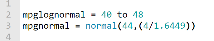
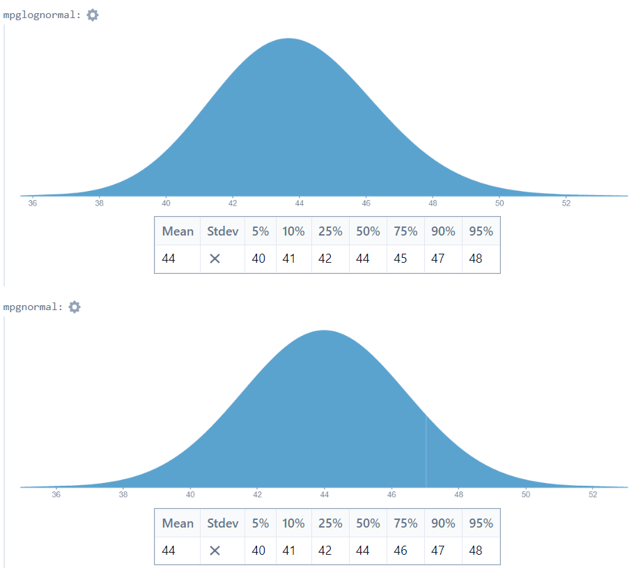
Turning to the Fuel Price example, we see that the normal/lognormal choice makes little difference when the ratio between interval bounds is small:
In this case lognormal and normal look very similar, and the distributions give means of 43.885 and 44 respectively.
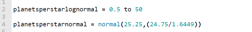
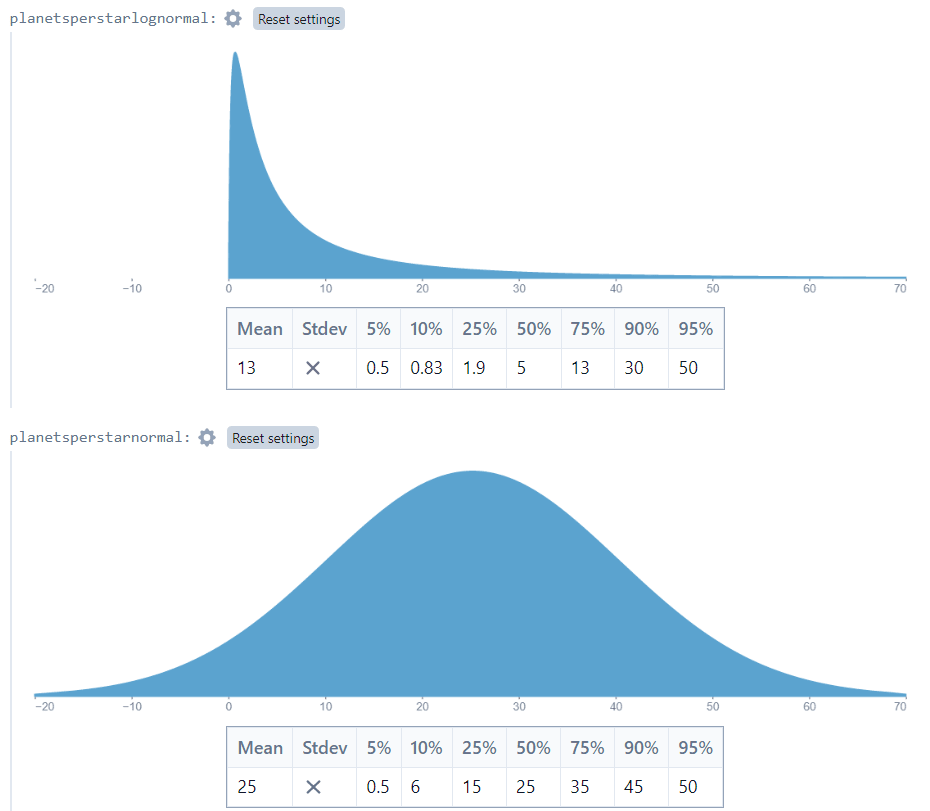
With the Inhabited Planets example, however, there is a different story. Using 0.5 and 50 as the 5th and 95th percentiles, I get very different-looking distributions:
The means are 13.32 and 25.25 for the lognormal and normal models respectively, and the shapes are very different.
Which is a better match for our understanding of the situation? In my opinion, the lognormal distribution is better. If we expect the number of planets per star to be between 0.5 and 50, the “expected” number of planets should be closer to 13 than to 25. Furthermore, the normal distribution assigns a nontrivial probability to (impossible) negative outcomes.
I think it’s clear that in this case the lognormal distribution is superior. But that’s just a gut feeling. Let’s explore this.
A high ratio between interval bounds implies positive skew
Consider datasets with a high ratio between the 5th and 95th percentiles:
The lengths of rivers (often used to exemplify Benford’s law)
The populations of cities/countries
Property prices
These all have positively-skewed distributions that could be approximated by the lognormal distribution.
Now consider broadly symmetric datasets:
The heights of adult males
The durations of pop singles
The price of gas in Florida gas stations today
These could probably be modelled with the normal distribution. Notice that in all of these cases, the ratio between the 5th and 95th percentiles will be low. A tall man is perhaps only 20% taller than a short man.
So in general a high ratio between 90% C.I. bounds implies positive skew and is hence better modelled by a lognormal distribution.
This isn’t a rigorous argument, but I suspect that you will struggle to think of examples that buck the trend. I can think of one. It’s possible that a normally-distributed variable could happen to have a small, positive 5th percentile. This would lead to a high ratio between 5th and 95th percentiles: suppose the temperature in my hometown has 5th and 95th percentiles of 0.1°C and 30.0°C respectively. The ratio between the bounds is 300, but the underlying distribution is probably symmetric and best modelled by a normal distribution. Note that the rule of thumb would apply if we measured temperature in Kelvin instead.
General findings: normal vs lognormal
The lognormal and normal distributions are similar when the ratio between interval bounds is low. The difference in means is just 3.6% when one bound is 2x the other.
The lognormal distribution is usually superior when the ratio between interval bounds is high. These circumstances usually imply negative skew, which make the lognormal distribution a better fit.
Although the lognormal is usually better, there are important considerations:
The lognormal distribution can only model positive values.
If you have reliable estimates of the mean and/or standard deviation of a distribution, the normal can be easier to model with.
Quantities with strict upper bounds (such as probabilities) may not be suitable for the lognormal distribution, although the normal distribution is usually not suitable either in these instances.
Not everything is positively-skewed or symmetric. The number of teeth in the next dental patient’s mouth, for example, would likely be positively skewed. But you could model “32 - number of teeth” as lognormal instead.
Creating aggregate estimates
In this section we will find that the "lognormal mean" can outperform the arithmetic mean, but may only be worthwhile in situations of high variability.
All else equal, modelling with distributions is better than using point-estimates. However we often don’t have reliable evidence for the shape of a distribution. This section explores the question: how can we use multiple point-estimates to create reliable aggregate estimates?
In this section I will consider three means:
The arithmetic mean
x1+x22
The geometric mean
2√x1,x2
The "lognormal mean": the mean of the lognormal distribution for which x₁, x₂ form an n% confidence interval. The lognormal mean will depend upon the size of this confidence interval.
Choice of mean should depend on the expected underlying distribution
Earlier we saw that estimating underlying distributions (rather than simply working with point-estimates) introduces personal bias. Our choice of mean is linked to our estimate for the shape of the underlying distribution, and unfortunately there is no way around it: each choice of mean makes an implicit assumption about the underlying distribution.
For simplicity, assume we have two sub-estimates which we wish to weight equally.
The arithmetic mean finds the mean of a symmetric distribution (such as the normal distribution) with symmetric confidence interval (x₁, x₂)
The geometric mean finds the median of any lognormal distribution with symmetric confidence interval (this is always lower th).
The lognormal mean finds the mean of a lognormal distribution with symmetric n% confidence interval (x₁, x₂)
The geometric mean is usually better than the arithmetic mean
Interestingly, it hardly matters which mean we use when the ratio between inputs is low.
Suppose, for example, that I have two estimates for the fuel-efficiency of my car.
The carmaker’s website claims 50mpg
My mechanic, who has experience with older models of my car, claims 40mpg
Type of mean used
Result
Arithmetic
45
Geometric
44.72
Lognormal, 68% C.I
45.004
Lognormal, 90% C.I
44.824
The four means differ by less than 1%.
The lognormal mean calculated from a 68% confidence interval is higher than the one calculated from a 90% interval. This is because the former distribution has higher standard deviation and therefore a bigger right tail.
What about when the sub-estimates are further apart? Let’s take two estimates for the number of planets per star in the galaxy: 1 and 10.
Type of mean used
Result
Arithmetic
5.5
Geometric
3.16
Lognormal, 68% C.I
6.18
Lognormal, 90% C.I
4.04
The arithmetic mean is now 74% greater than the geometric mean, and the lognormal mean calculated from a 68% confidence interval is nearly double the geometric mean. Once again, it’s the ratio between inputs that matters here. When the ratio is low, the means are close. When the ratio is high, the means diverge.
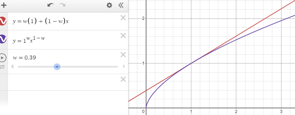
I built a tool to explore this further. x represents the ratio between the two sub estimates (x₂/x₁) and p represents the size of the confidence interval used to generate the lognormal mean.
Try moving p towards 1: you will see that the lognormal mean tends to the geometric mean.
So which mean is better when the ratio between inputs is high? In the last section we saw that a high ratio between C.I. bounds implies a positive skew. It follows that a high ratio between sub-estimates also implies a positive skew in the underlying distribution.
Clearly the arithmetic mean (which assumes an symmetric underlying distribution) is no good in this scenario.
The geometric mean is essentially the lognormal mean formed by a 100% confidence interval. If we have reason to believe x₁, x₂ are extreme outliers (worst- and best-case estimates, say) then this could be a good choice.
The lognormal means are viable candidates, but they vary considerably based on the assumed size of the confidence interval used. If we have no objective evidence for the size of the confidence interval, we have to use subjective judgement to decide the size.
Of course, the underlying distribution may be neither normal nor lognormal. As uncertainty increases the distribution of the long tails become increasingly influential on the mean. But I won't explore other tail types here.
In short, it makes sense to assume a lognormal distribution when the ratio between sub-estimates is high, and hence a lognormal mean is a good choice. However this requires a judgement call on the size of the confidence interval represented by x₁, x₂.
If you want a rule of thumb, it may make sense to generate lognormal means from a 90% confidence interval by default. As long as the ratio between sub estimates is under 1000, the lognormal mean will lie roughly midway between the geometric and arithmetic means: a good compromise. The main worry should be that you are ignoring the effects of an undetected fat tail.
Here's how I would apply the above to my two key examples.
Fuel Cost example:
I have two estimates for the fuel-efficiency of my car.
The carmaker’s website claims 50mpg
My mechanic, who has experience with older models of my car, claims 40mph
It seems reasonable that these estimates represent best- and worst-case estimates for the true fuel efficiency of my car, so I suspect the geometric mean (or, similarly, lognormal mean using 99% C.I of (40,50)) will be most accurate. However, since the ratio between estimates is low, I opt for the simpler arithmetic mean, 45.
Inhabitable Planets example:
An astronomy paper claims that "stars in our galaxy probably have on average 1 to 10 planets each".
The source gives no confidence intervals, but I choose to interpret "probably" as 90% confidence, and hence use a 90% confidence interval to generate a lognormal mean of 4.04 planets per star.
Weighted means
Sometimes we have multiple point-estimates and varying levels of confidence in each one. So we use a weighted mean to build an aggregate estimate.
The thought of weighted lognormal means is exploding my brain at the moment, so I will stick to weighted arithmetic and geometric means, which are very straightforward.
We apply weights w1+w2+...+wn to our sub-estimates x1+x2+...+xn to build an arithmetic weighted mean:
x=w1x1+w2x2+...+wnxn where w1+w2+...+wn=1, w∈[0,1]
The equivalent for the geometric mean is
x=wx11wx22...wxnn where w1+w2+...+wn=1, w∈[0,1]
As with the unweighted means, the weighted arithmetic and geometric means are close when the ratios between estimates are low. The graph shows the two-estimate example, where the x-value is the ratio between the sub-estimates:
Again, I would argue that the geometric mean is generally superior. When the sub-estimates are close it hardly matters, and when they are far apart the geometric mean better captures the positive skew in the underlying distribution.
General findings: aggregate estimates
When the ratio between the inputs is <3, the arithmetic, geometric and lognormal means are similar. Since the arithmetic mean is more widely understood, it may be a better choice when the ratio between inputs is low.
As the ratio between inputs grows, the means diverge. The high ratio suggests underlying positive skew, which makes the arithmetic mean unreliable. A judgement call is needed to estimate the size of the confidence interval represented by our inputs, which introduces subjectivity. One way to avoid this is to state in advance that you will use 90% lognormal means in place of unweighted arithmetic means of two values.
The geometric mean can be thought of as the mean of a lognormal distribution for which the inputs form extreme outer limits
We have not explored how to apply the lognormal mean in situations with three or more inputs, or with weighting
Conclusion: complexity vs legibility
We have seen a common theme throughout: simple methods show high fidelity in situations of low variability (as measured by the ratio between confidence interval bounds or of sub-estimates).
So I would make the following suggestion: If your work is for public scrutiny, needs to avoid subjectivity or is time-sensitive, only use the more complex methods when it makes a significant difference.
Point estimates are fine if your final calculation is not too long and the ratio between 90% confidence interval bounds is less than 2 (or if you don't need to divide by an unknown and you don't care about the "shape" of your answer).
The normal distribution is easier to understand than lognormal, so favour it when the ratio between confidence interval bounds is low
The arithmetic mean is widely understood, so use it as long as most of the inputs vary by less than a factor of 2
On the other hand, simple methods can lead to spurious results in situations of super-high variability. For example, estimates for the incidence of intelligent life in the galaxy (a high variability, multi-stage calculation) vary wildly depending on the complexity of the methods used.
Thanks to the makers of Squiggle, which has made working with more complex models much faster.
Changes
[23 Mar] Amended point-estimate section to reflect that multiplication is fine with point estimates, while division introduces error. Changed summaries accordingly. Thanks to @Thomas Sepulchre (LessWrong) for the comment.
[27 Mar] Corrected errors on Squiggle graphs that compare similar lognormal/normal distributions - I had been using the wrong standard deviations for the normal distributions before.
[1 Apr] Brought work on the lognormal mean into the post and ceased to interpret its sensitivity to heavy right-tails as a sign of unreliability. Added more on the pros and cons of using interval estimates as inputs and outputs. Thanks to @Vasco Grilo for feedback.
[3 Apr] Re-wrote the section "Should we always use interval estimates?" to separate the question of using interval estimates for inputs vs outputs, and to add examples.


 Again, I would argue that the geometric mean is generally superior. When the sub-estimates are close it hardly matters, and when they are far apart the geometric mean better captures the positive skew in the underlying distribution.
Neat post, and nice to see squiggle in the wild.
Some points
You could create a mixture distribution, you could fit a lognormal whose x% confidence interval is the range expressed by the points you've already found, you could use your subjective judgment to come up with a distribution which could fit it, you could use kernel density estimation (https://en.wikipedia.org/wiki/Kernel_density_estimation).
In your number of habitable planets estimate, you have a planetsPerHabitablePlanet estimate. This is an interesting decomposition. I would have looked at the fraction of planets which are habitable, and probably fit a beta distribution to it, given that we know that the fraction is between 0 and 1. This seems a bit like a matter of personal taste, though.