People more involved with X-risk modelling (and better at math) than I could better say whether this is better than existing tools for X-risk modelling, but I like it! I hadn't heard of the absorbing state terminology, that was interesting. When reading that, my mind goes to option value, or lack thereof, but that might not be a perfect analogy.
Regarding x-risks requiring a memory component, can you design Markov chains to have the memory incorporated?
Some possible cases where memory might be useful (without thinking about it too much) might be:
How well past social justice movements went may have implications for the success of future movements that relate to X-risk
The way in which problems end may have implications for future problems
Maybe this information can just be captured without memory anyway?
A fully generic Markov chain can have a state space with arbitrary variables, so can incorporate some memory that way. But that ends up with a continuous state space which complicated things in ways I'm not certain of without going back to the literature.
An easier solution is if you can consider discrete states. For example, ongoing great power war (likely increases many risks) or pandemic (perhaps increases bio risk but decreases risk of some conflicts) might be states.
I think to properly model Ord’s risk estimates, you have to account for the fact that they incorporate uncertainty over the transition rate. Otherwise I think you’ll overestimate the rate at which risk compounds over time, conditional on no catastrophe so far.
Thanks for writing this up Ismam! It seems comprehensive and useful (albeit to a complete novice). In particular, time-inhomogeneity seems very useful to model.
Is knowledge of/aptitude with CTMC common among actuaries?
Also, have you considered doing some more work to apply it to ER with expert support?
Related to both questions, I'd like to see new approaches like this (e.g, which consider time-inhomogeneity) applied to prioritising existential risk and other causes.
One reasons for that is because I think that a lot of the differences between how EAs and others view the priority of climate change is underpinned by different expectations around the linearity of the growth of risk over time (e.g., relative to other concerns like AI). It would therefore be great to see someone dive into that more.
My interest is probably not a high quality signal of demand though!
Is knowledge of/aptitude with CTMC common among actuaries?
Yes, it's required learning for actuaries, they may just need to brush up on their lecture notes.
Also, have you considered doing some more work to apply it to ER with expert support?
Absolutely. I think, before I embark on further work, I would really like to talk with cause prioritisers/grant-makers to confirm that they would have confidence in this kind of modelling, and to understand what kinds of outputs they would value.
Very much agree RE time-inhomogenous. Some people may see them as a bug (fair) but in many ways they are a feature. I've said in the post that CTMCs can help disagreeing X-Risk modellers understand the precise source of their disagreements (ie differing time-inhomogeneity assumptions).
Apologies, I could have made this clearer. It is only those diagonal entries which are allowed to be negative. In fact they must be negative (or zero).
Technically, the diagonal entries are transitions from state i to i (ie. they are not really transitions but rather a measurement of "retention"). You can think of the positive or negative sign as indicating if it is a measure of transitioning away from the state, or retention in the state.
This is a crosspost from the new Animal Welfare Alignment Newsletter by Anima International. You can subscribe on Substack if you are interested in following these efforts. Audio reading also available on Substack.
The goals of this post are to:
1. Raise a question I see as crucially important to the goal of aligning AI to animal welfare...
I used AI to fix transcription errors, rerrarange the ideas, and suggest tweaks to the title and some sentences.
Three of the most exciting projects to come out of EA in recent years are, in a vague sense, CEA spinouts:
* Kairos is directly a spinout of CEA and now handles most support for university AI safety groups. Basically everyone I've found who knows them is really excited about what they do
* NEST is an opinionated ideas-fi...
Hello! I'm Justin Portela. I got hired by GWWC to make YouTube videos after AI in Context did such a kickass job.
My channel is using that same cinematic, high-production value beauty to talk about everything in the EA universe that isn't AI.
...
TLDR; CTMCs are a mathematically accurate way of modelling X-Risks. Skip to section X-Risk Model using CTMCs to see the results of a model I performed using Toby Ord's estimates in The Precipice.
Purpose
Continuous-Time Markov Chains (CTMCs) are a popular tool used throughout industry (e.g. insurance, epidemiology) and academia to model multi-state systems.
In this post, I discuss how CTMCs have desirable features that make them well-suited to model Existential Risk (X-Risk) scenarios. I then produce a model based off of Toby Ord's probability estimates (The Precipice) for demonstration purposes.
By specifying a system of X-Risks and probability assumptions such as Ord's, I show how mathematical solutions can be derived to understand the implications of the system of assumptions.
The Total X-Risk Probability
Marginal Reduction in Total X-Risk from eliminating one risk
Expected time until extinction
Likeliest X-Risk at any given moment in time
Two applications of CTMCs I discuss in this post are:
Informing cause prioritisation decisions
A method to sense check and revise probability estimates
I am able to derive some results, and provide my suggestions on interpretation and application.
I also discuss limitations and weaknesses of CTMCs, and provide a brief comparison to alternative modelling approaches.
Mathematical Pre-requisites
This is a very maths-heavy forum post, but please don't get intimidated by the technical mathematical derivations which are not important to understanding the final results.
My hope is that most readers interested in X-Risk models are able to takeaway the main points about the capabilities of CTMC modelling, only requiring an understanding of:
probability concepts (e.g. dependent vs independent probabilities)
X-Risk scenarios
But to readers wishing to conduct CTMC modelling themselves and follow the mathematical derivations, you will need to have an understanding of
probability distributions
ordinary differential equations
matrix exponentiation
markov chains
Readers with actuarial, biostatistics, or similar backgrounds may meet many of these pre-requisites, and indeed CTMCs are applied in these fields. I personally have an insurance/actuarial background, and was inspired by those techniques used in industry.
CTMCs are used to model a system with multiple states, where transitions can take place at any point in time from one state to another.
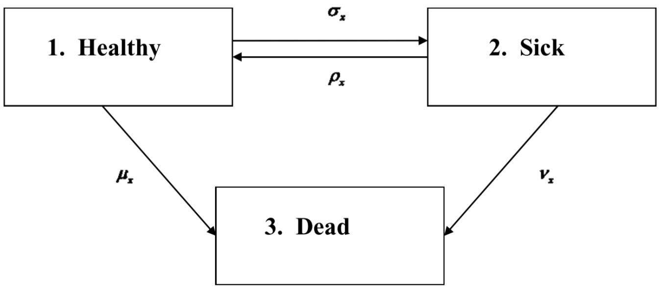
To familiarise readers to the concept of CTMCs, here I introduce the Health-Sickness-Death (HSD) model, and talk through some core CTMC concepts. This is a popular model used to model hospital patients.
ACST355 Lecture Notes 2016S1 Macquarie University
In the above example, there is one absorbing state (Death) and two non-absorbing states (Healthy and Sick). The patient can move back and forth between the non-absorbing states indefinitely. Once in the absorbing state (Dead) however, there can be no further transitions. This is indicated in the diagram by the absence of arrows pointing outwards from the Death state.
The notation used for the probability of transitioning from one state to another (e.g. Healthy to Dead) is: P(State at time x+t =Dead| State at time x = Healthy)=pHDx(t).
The Greek letters (e.g. μx) are transition intensities, which I like to think of as "instantaneous probabilities" that a patient moves from one state to another. They're not real probabilities as they sum to zero/ can be negative/ can exceed 1, but that hasn't stopped me from thinking of them as such. Transition intensitiesare a core concept in CTMCs, and later I explain how they help modellers think about risks more clearly.
Their formal definition is: μx=limh→0pHDx(h)h.
The subscript x here refers to the age of the patient. And so these transition intensities in this HSD model themselves can be functions of age (or time). Such Markov Chains are described as being time-inhomogeneous. This is important to account for as we know older patients have higher death rates (e.g. μ70>μ30) than younger, and hence it would be inaccurate to use constant (time-homogeneous) intensities.
The intensities can be collected together and written into matrix form:
A(x)=⎡⎢⎣−(σx+μx)σxμxρx−(ρx+νx)νx000⎤⎥⎦ Note that the diagonals aii=−∑j≠iaij so that each row sums to zero.
By generalising for any two states (m,n), and taking the limit, we can arrive at a set of differential equations known as the Kolmogorov forward equations:
ddtpmnx(t)=limh→0pmnx(t+h)−pmnx(t)h=∑jpmjx(t)σjnx+t , where σ are our transition intensities. This can also be expressed in matrix form:ddtP(t)=P(t)A(t)
This a system of ordinary differential equations that can be solved simultaneously. The solution is P(t)=e∫txA(t)dt, where "e" is the matrix exponential operator.
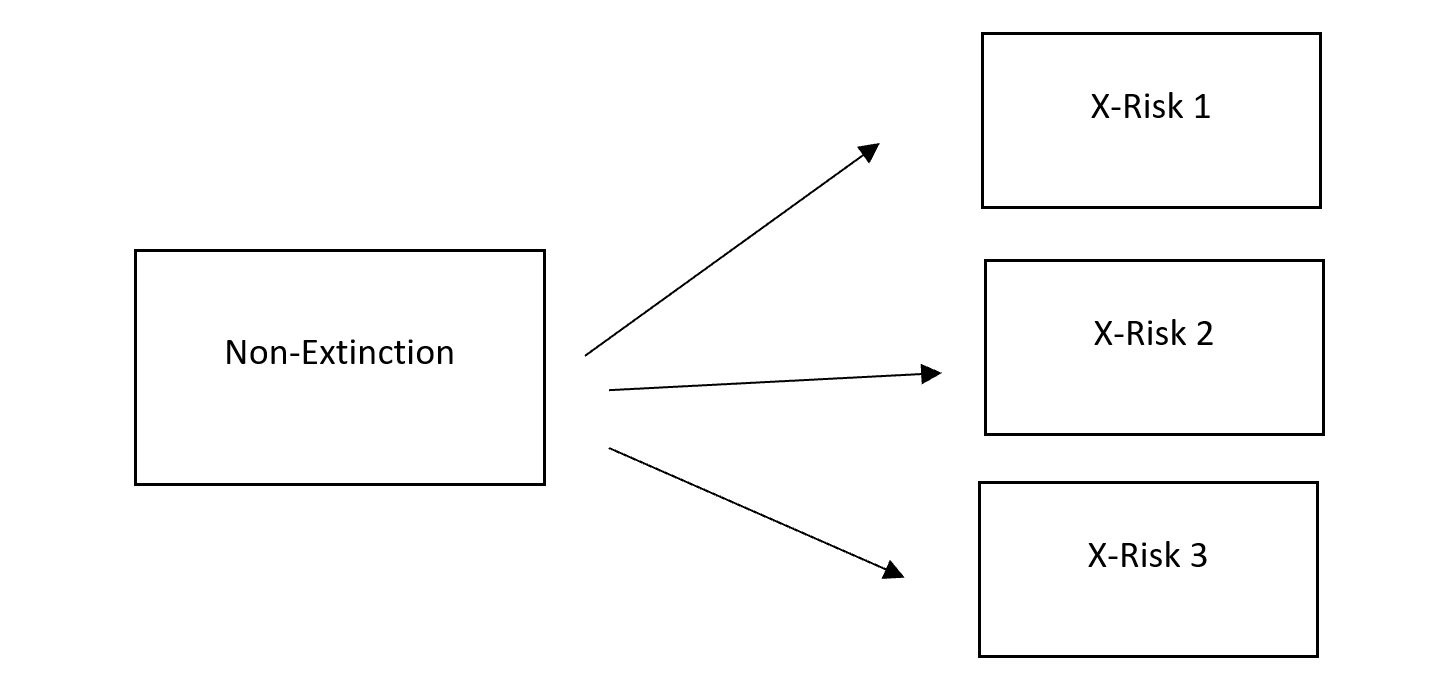
Similar to the Health Sickness Death Model, we can create a multi-state model for X-Risk scenarios. The special feature of X-Risk systems is that there are multiple absorbing states due to the multiple X-Risks.
To demonstrate, here I apply CTMCs to Toby Ord's estimates in The Precipice.
First I reverse-engineer Ord's probability estimates into transition intensities. I then assign an assumption (e.g. constant, exponential) about how each risk changes with time (time-inhomogeneity effects). Generally speaking, natural risks have constant intensities as the risks are independent of time. Anthropogenic risks however tend to vary with time owing to heightened periods of political tension, changing climate effects, and advances in technology etc.
The time-inhomogeneity assumptions I assign are my own and I don't wish them to be taken as serious recommendations. Properly informed assumptions can definitely be made by consulting with relevant experts for each X-Risk (e.g. Climate change researchers).
X-Risk
Ord's Probability Estimates over 100 years (q)
Assumed Relationship with Time
(Demonstration Purposes only)
Implied Transition Intensity (μt)
Asteroid or comet impact
0.000001
Constant
1×10⁻⁸
Supervolcanic eruption
0.0001
Constant
1×10⁻⁶
Stellar explosion
0.000000001
Constant
1×10⁻¹¹
Nuclear war
0.001
"Normal" plus baseline. Peak risk is twice baseline risk, occurring in 20 years (≈2050).
2.01×10⁻⁴(1√2π×102+ dnorm(mean = 30, std = 10))
where dnorm is the pdf of the normal distribution.
Climate change
0.001
Risk doubles every 10 years
6.78×10−8×20.1t
Other environmental damage
0.001
Constant
1×10⁻⁵
'Naturally' arising pandemics
0.0001
Constant
1×10⁻⁶
Engineered pandemics
0.033333333
Constant
3.39×10⁻⁴
Unaligned artificial intelligence
0.1
Risk doubles every 5 years
7.14×10−6×20.2t
Unforeseen anthropogenic risks
0.033333333
Constant
3.39×10⁻⁴
Other anthropogenic risks
0.02
Constant
2.0×10⁻⁴
We can also calculate the dependent probabilities for each X-Risk using this result:
pix(t)=μix∑jμjx−μix+t∑jμjx+te−t∫0∑jμjx+tdt
Note this equation is for the case when there is only 1 non-absorbing state. If you have multiple non-absorbing states you will need to re-solve the matrix exponential equation: P(t)=e∫txA(t)dt with the appropriate transition matrix A(t). The HSD model for example has 2 non-absorbing states and hence a different equation which I quote in the HSD section.
Dependent probabilities (p) This is the probability of the particular X-Risk occurring with consideration of all other X-Risks. A full description of the space of all possible X-Risks is required to calculate these estimates.
Independent probabilities (q) In contrast, independent probabilities only require judgement of the particular X-Risk in isolation, without consideration of other existential risks and how they may compete and interact. As such these probabilities are easier to assign and work with.
Selected X-Risks
Ord's Independent probability estimate over 100-years q0(100)
Implied Dependent probability over 100 years p0(100)
Supervolcanic eruption
0.0001
9.42×10⁻⁵
Nuclear war
0.001
9.49×10⁻⁴
Climate change
0.001
8.79×10⁻⁴
And here are the results.
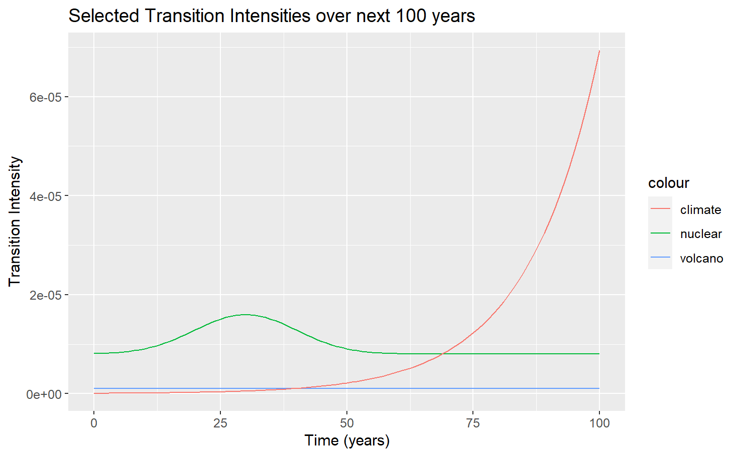
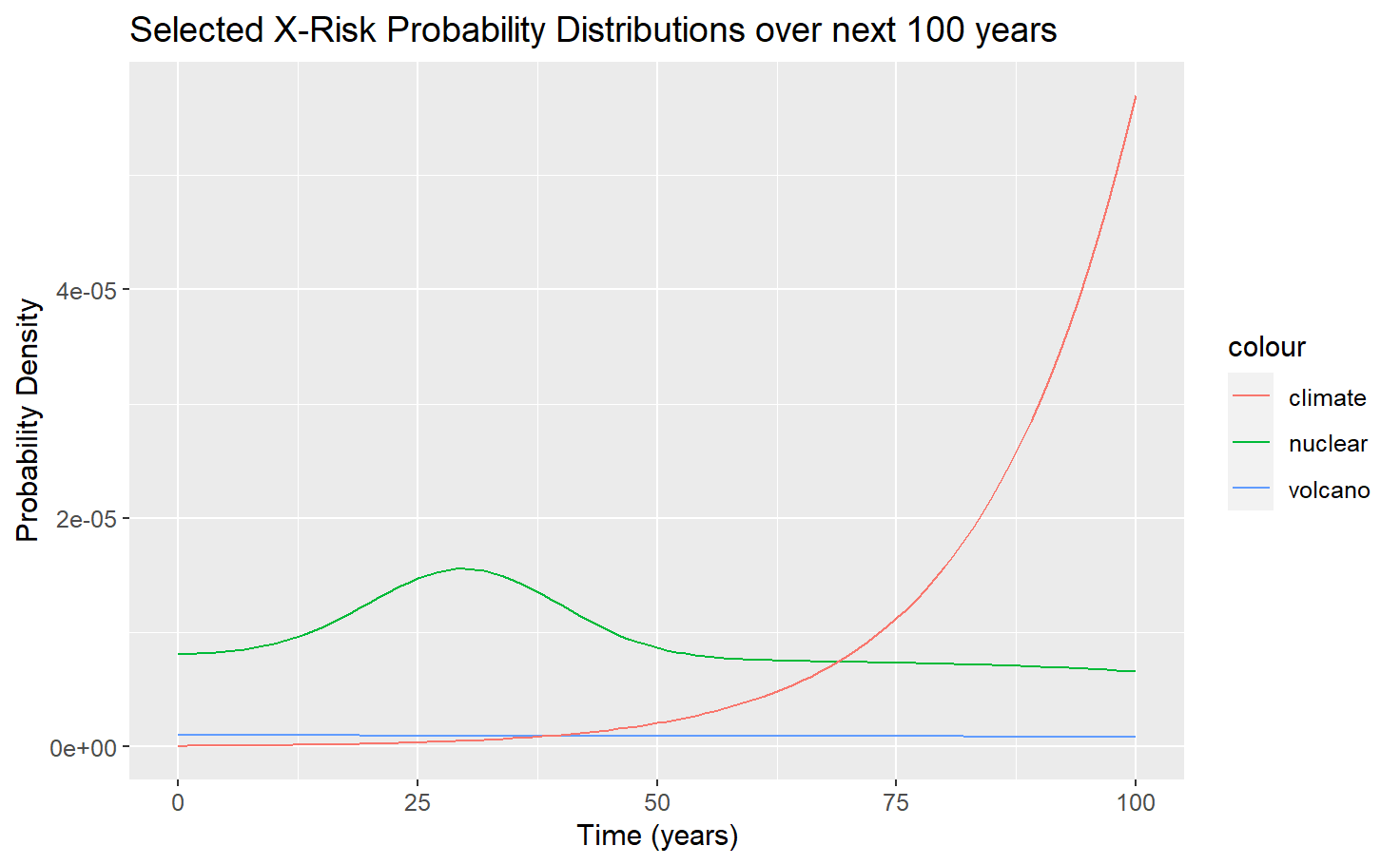
Transition intensities and probability density
What we can see is how X-Risks evolve with time and compete with each other over the next century.
Notice that the probability density distributions are similar to the intensities but angled slightly downwards, (most visible in Nuclear War). What's happening is that the CTMC maths is taking into account the small but growing probability that an X-Risk event has already taken place.
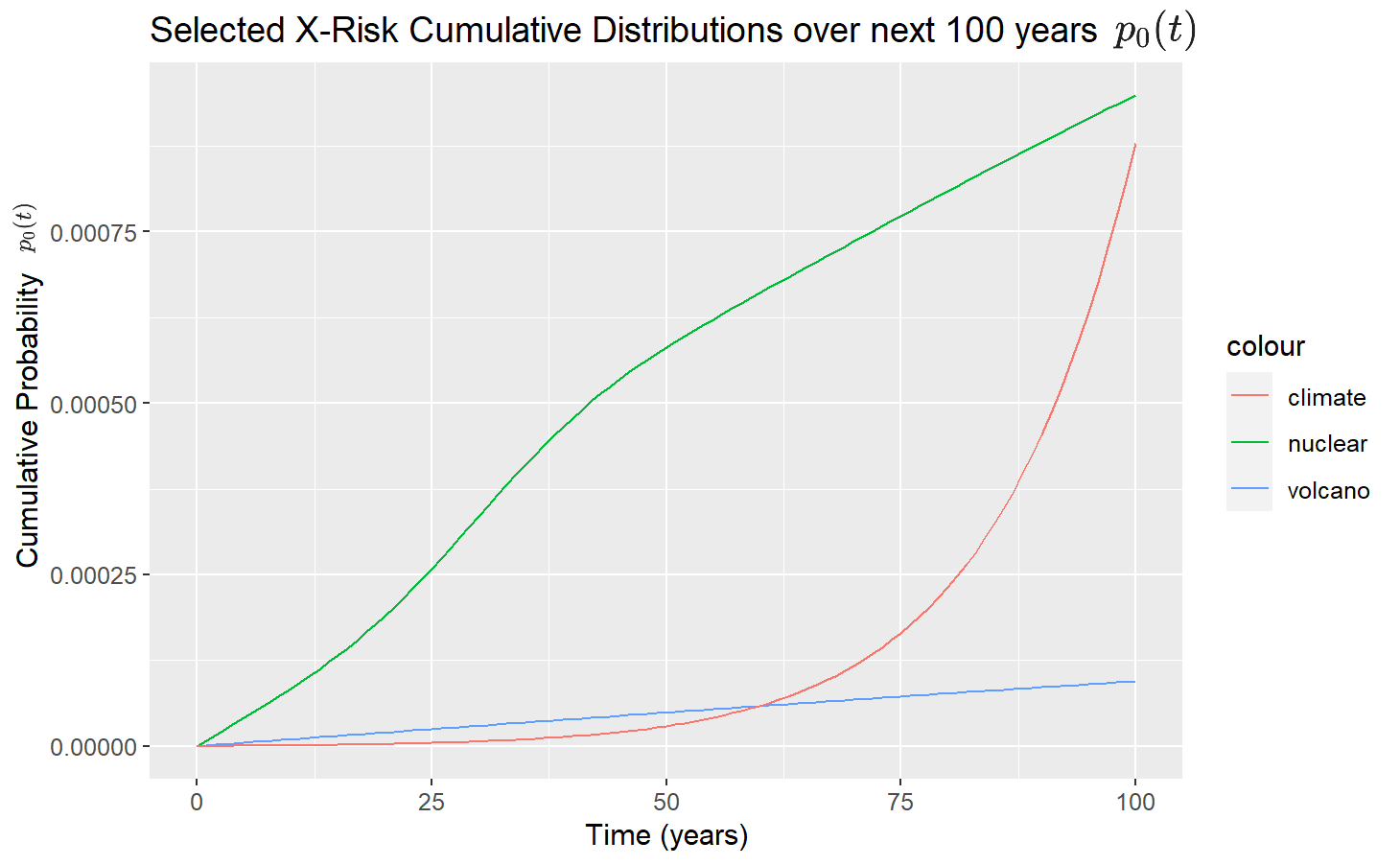
Cumulative probability
Notice that Ord's estimate for Climate and Nuclear in 100 years is the same, i.e. qnuclear0(100)=qclimate0(100)=0.001. However, this chart shows that nuclear is slightly higher at 100 years. What's happening is that Ord's estimates are "independent" (q) estimates that treat each X-Risk in isolation. But with CTMCs, we can calculate the "dependent" probabilities (p), and since the time assumptions I gave nuclear give it a higher chances of happening in the earlier part of the century, it ultimately has a slightly higher value by year 100.
This demonstrates a very powerful application of CTMCs in cause prioritisation. For example grant-makers are often deciding to allocate resources now, and may consider many measures in their decision-making:
reducing total X-Risk
reducing X-Risks over the next 100 years
maximising Expected-Life Years
A grant-maker may decide Nuclear is more important to reduce because it provides both long-term and immediate benefits.
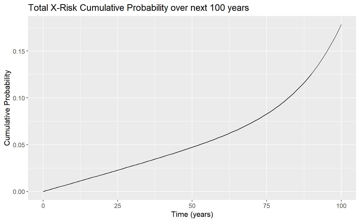
Total X-Risk
We can calculate the TotalX-Risk probability as such:pTotalx(t)=∑ipix(t)=1−e−∫t0∑jμjx+t∗dt∗=1−∏j(1−qjx(t)) This result is not unique to CTMCs and is quoted in Ord's book The Precipice. But it does show that CTMCs are consistent with conventional probability calculations.
We can calculate the Expected Time until an X-Risk event:
E(T)=∞∫01−pTotal0(t)dt
Just be careful that the time assumptions continue to be sensible beyond 100 years. For example I assumed that the Climate and AI risks (ie transition intensities) respectively became zero and constant after 100 years, as they were exponential and would have approached inifity with time.
This was my result: 194.31 years.
We can also calculate Expected Life-Years lived by human beings using this result:
E(LY)=∞∫0(ddtpTotal0(t))∗WorldPopulation(t)dt
Population projections can be used from sources like the UN (albeit not to infinity). I have not performed such a calculation but am confident it is doable.
We can also calculate the net reduction in Total X-Risk from eliminating or mitigating one X-Risk.
NetReduction in Total X-Risk Probability(t)=pTotalx(t)originalmodel−pTotalx(t)newmodel
This was my result, if Nuclear War is eliminated as an X-Risk: NetRedcution (100 years) = 0.1784552 - 0.1776329 = 0.0008223671
Note that this value is slightly less than the probability of a nuclear war happening, pNuclear0(100)=0.000948905. This is because when one X-Risk disappears, the other X-Risks step in to "compete" for the freed up territory.
Similarly, we can also calculate: Net Improvement in Years Saved = E(T)originalmodel−E(T)newmodel
Further Advanced Models
Here I speculate about possible further advanced models.
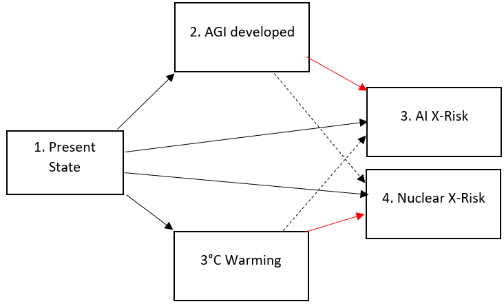
Elevated States
We can add further non-absorbing states to our models, to incorporate "elevated states" if we think it is important to model states which exacerbate the chance of X-Risk, whilst not being X-Risks themselves. For example, we may suppose that 3°C warming increases the likelihood of global conflict and nuclear war. These elevated states play a similar role to the Sickness state, in the HSD model. They may align the model closer to reality.
Red lines to signify increased risk of transition
Multivariate transition intensities
I also wonder if it is possible to model transition intensities as multivariate functions. For example I would love to model the climate and nuclear intensities as functions of time and CO2 levels. Then it would be possible to rely on an explicit CO2 projections which would be superior to the example I gave using "elevated states". Unfortunately I cannot find any literature on such models.
Discrete effects
It is also possible to introduce "discrete effects" into the model for X-Risk events that may only take place at a known fixed point in time (e.g. date of a gender reveal party with universe-ending potential).
Incorporating uncertainty
It should also be possible to embed uncertainty into these models allowing models to show the degree of confidence/uncertainty, including the usage of confidence intervals/ prediction intervals. Here I suggest two ways.
We can assign a distribution (Bayesian credence) to the initial probability estimates (or transition intensities) and use monte-carlo simulations.
I also wonder if it is possible to model transition intensities as random processes (e.g. random walk/ brownian motion). We can then make it so our certainty in risks decreases with time, reflecting greater uncertainty in the far future.
Applications
Cause Prioritisation
As discussed in the results section, CTMCs can produce many results that would be of interest to cause prioritisation research.
Total X-Risk
How X-Risks emerge and compete over time
Expected Life-Years
These are highly relevant statistics to prioritisers. Prioritisers for example would be interested in estimating the effect of a potential intervention. Using CTMCs, they can estimate the marginal reduction in Total X-Risk, or Expected Life-Years, of different interventions.
They could even produce figures like Expected "Life-Years" saved per dollar, a quantity that is analogous to QALYs/DALYs per dollar used by charity evaluators like GiveWell.
It's important not boil everything down into a single number (expected value/mean), and consider a wide variety of statistics (median, 95th percentile etc) and the distributions themselves. CTMCs can provide these.
CTMCs can even help cause prioritisers decide when to target their intervention, by targeting peak periods of risk when the intervention would be most effective.
There are lots of possibilities in this area.
Sense-checking probability estimates
CTMC models use probability estimates such as Ord's as inputs. But, by reversing this process, CTMCs are also useful to sense-check if these estimates were reasonable in the first place. If our CTMC model produces silly results, it's usually because of flawed assumptions.
Transition intensities, a core concept in CTMCs, can also help modellers think about X-Risks in a clarified way because of three properties:
Transition intensities are independent Unlike probability estimates which come in dependent and independent forms, intensities are always independent.
Transition intensities are local Probabilities (density or cumulative), are non-local. They are calculated over a window of time (x,t).
Transition intensities are linear Unlike probabilities, intensities are linear. If we have two X-Risks with intensities μ1 & μ2, and we suppose that one is twice the other (i.e. μ2=2μ1), then we are supposing that in a small window of time (e.g. a day), X-Risk #2 is twice as likely to take place. This is also true for the same X-Risk at different points of time (e.g. AI today, vs AI in 10 years). Using a small window of time allows for us to think about risks linearly. This is helpful since over a long timeframe, non-linear effects arise. Thus it is often advantageous to think about risks first in terms of transition intensities.
In the weakenesses section on time-inhomogeneity, I also explain that transition intensities can help disagreeing X-Risk modellers understand the precise source of their disagreement better, and improve the quality of debate.
Advantages and Weaknesses of CTMCs
Advantages
CTMCs have many desirable features ready-made, that address important needs in X-risk modelling.
Continuous Time Markov Chain Feature
Relevance to X-Risk modelling
Multiple Absorbing States
Multiple competing X-Risks.
Multiple non-absorbing states
Ability to incorporate Elevated States (e.g. 3°C warming scenario) that modify and interact with other X-Risks but are not themselves X-Risks.
Time-dependent transition intensities
Ability to assume X-Risk probabilities vary with time.
They capture important probability concepts in a mathematically accurate way that is often missed by other approaches.
Marginally decreasing Total X-Risk probability due to X-Risks competing with each other
Independent vs dependent probabilities
Marginally diminishing X-Risk probability density over time, as an X-Risk may have already occurred
In my opinion, CTMCs can reveal unintuitive results accurately that often missed by less sophisticated models.
CTMCs are well-studied in academic literature and established industry methods in insurance and biostatistics. There are well documented guides and lecture notes on CTMCs. There are maintained pacakges in R, Python & Julia for CTMC modelling, as well as the underlying mathematical techniques (integration, matrix exponentiation etc).
CTMCs are also able to produce analytical (exact) mathematical solutions, instead of numerical approximations. This is more of a nice-to have feature. It allows us to present results, and analyse results with calculus techniques.
Weaknesses and Limitations
Time-inhomogeneity assumptions
Assigning time-inhomogeneity assumptions to transition intensities is half art and half science. It is very similar in this sense to assigning probability estimates to X-Risks. Assumptions are contentious and indeed political. Different experts/modellers will have different views and different intuitions.
In my opinion, all X-Risks models are making an assumption on how X-Risks evolve with time, it's just that it's often implicitly. CTMCs simply make the assumptions explicitly and obvious. I do think the transition intensities ultimately help modellers understand exactly what their intuition is saying (e.g. Risk doubles every n years, natural X-Risks are constant), and so it should help improve the debate amongst disagreeing modellers as they can pinpoint their precise difference.
Memorylessness
A core assumption of Markov models is that they are memoryless (the Markov property). This means that the future (i.e. the transition intensities) only depends on the current state, and not the history of previously occupied states. Assuming the markov property greatly simplifies modelling but will be a severe flaw in the model if non-memoryless effects are material. This is a known flaw in the Health-Sickness-Death Model since patients that occupy the Sick state for prolonged periods of time are likelier to die.
Every X-Risk that I can think of is memoryless and so I do not think this is a problem. I tried to think of what memory would look like and the best I could think of is this: possibly a period of prolonged occupation in an "elevated state" (3C warming) may increase increases X-Risks more than fleeting occupation of the "elevated state". Even in this scenario, I feel that the memory effects are very minor. But I encourage readers to think about possible memory effects.
These concepts need to be overlaid onto CTMCs, perhaps with other models/frameworks.
Comparison of CTMCs to alternate approaches
Discrete Markov Chain Models
Discrete Markov Chains use discrete, equally-spaced time units instead of continuous results. CTMCs are their natural analogue/ generalistion. It is common practice to approximate continuous-time effects by using many discrete small time-intervals. I fully expect discrete models to produce similar results (albeit slighlty off). This can be a good way to check two models are correctly working.
Another approach to model X-Risks is to assume there is a constant probability of an X-Risks event happening in any year (Geometric distribution) or moment in time (Exponential distribution).
These models are simple and straightforward, and perfectly adequate for certain use cases. But they are not able to capture time-inhomogeneity effects.
This approach is actually a special case of CTMC approach (where we assume constant risk), and the exact same results are arrived at (an exponential distribution of T∼Exp(∑jμj)).
Toby Ord's model in The Precipice uses a fixed time period of 100 years. With this model and his arrived at estimates, he is able to produce a calculation of Total X-Risk probability using probability theory, and discuss dependent vs independent probabilities and how X-Risks compete with eachother.
The main drawback of these models is that they are inflexible if wishing to use a different time period. They are effectively a discrete markov chain model of 1 time step.
I point out in this post that Ord's Total X-Risk probability calculation is reproduced with CTMCs, pTotalx(t)=1−∏j(1−qjx(t)). This gives me confidence that CTMCs are indeed a generalisation this approach.
Acknowledgements
Special thanks to Emrik Garden, Arepo (Sasha Cooper), Kramer Thompson, Sam Nolan, Rumi Salazar, Riley Harris, Bradley Tjandra for their assistance with this post.


Oooh, this is sexy. Thanks for writing it!