Comments
Five slightly more hardcore Squiggle models.

Following up on Simple estimation examples in Squiggle, this post goes through some more complicated models in Squiggle.
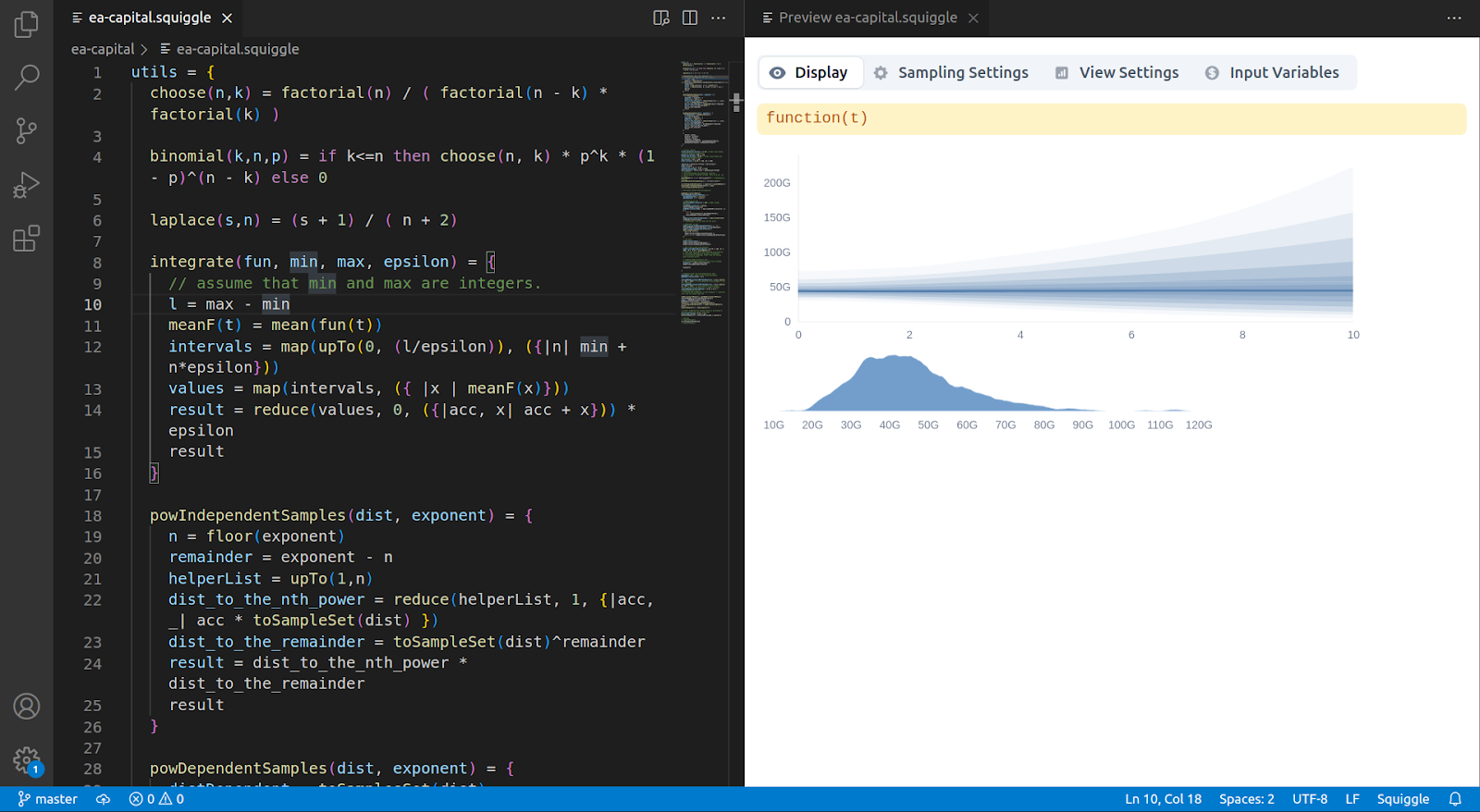
As well as in the playground, Squiggle can also be used inside VS Code, after one installs this extension, following the instructions here. This is more convenient when working with more advanced models because models can be more quickly saved, and the overall experience is nicer.
Recently, when talking about AI timelines, people tend to give probabilities of AGI by different points in time, and about slightly different operationalizations. This makes different numbers more difficult to compare.
But the problem with people giving probabilities about different years could be solved by asking or producing probabilities for all years. For example, we could write something like this:
// Own probability
_sigma(slope, top, start, t) = {
    f(t) = exp(slope*(t - start))/(1 + exp(slope*(t-start)))
    result = top * (f(t) - f(start))/f(start)
    result
}

advancedPowerSeekingAIBy(t) = {
    sigma_slope = 0.02
    max_prob = 0.6
    first_year_possible = 3

    // sigma(t) = exp(sigma_slope*(t - first_year_possible))/(1 + exp(sigma_slope*(t-first_year_possible)))
    // t < first_year_possible ? 0 :  (sigma(t) - sigma(first_year_possible))/sigma(first_year_possible)*max_prob
    sigma(t) = _sigma(sigma_slope, max_prob, first_year_possible, t)
    t < first_year_possible ? 0 : sigma(t)
}
instantaneousAPSrisk(t) = {
    epsilon = 0.01
    (advancedPowerSeekingAIBy(t) - advancedPowerSeekingAIBy(t-epsilon))/epsilon
}

xriskIfAPS(t) = {
    0.5
}

xriskThroughAps(t) = advancedPowerSeekingAIBy(t) * xriskIfAPS(t)
This produces the cumulative and instantaneous probability of “advanced power-seeking AI” by/at each point in time:
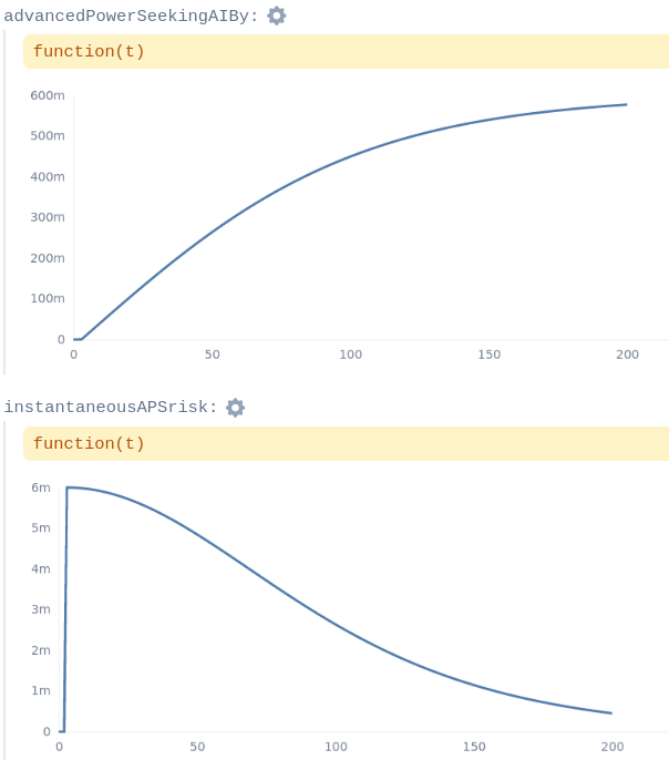
And then, assuming a constant 95% probability of x-risk given advanced power-seeking AGI, we can get the probability of such risk by every point in time:
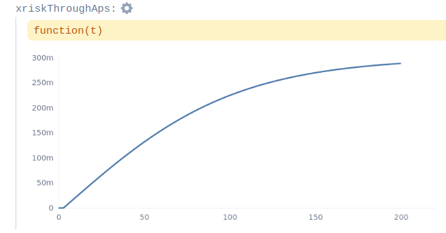
Now, the fun is that the x-risk is in fact not constant. If AGI happened tomorrow we’d be much less prepared than if it happens in 70 years, and a better model would incorporate that.
For individual forecasts, rather than for models which combine different forecasts, <forecast.elicit.org> had a more intuitive interface. Some forecasts produced using that interface can be seen here. However, that interface is currently unmaintained. Open Philanthropy has also produced a number of models, generally written in Python.
In the preceding post, I presented some quick relative estimates for possible career pathways. Shortly after that, Benjamin Todd reached out about estimating the value of various career pathways he was considering. As a result, I created this more complicated spreadsheet:
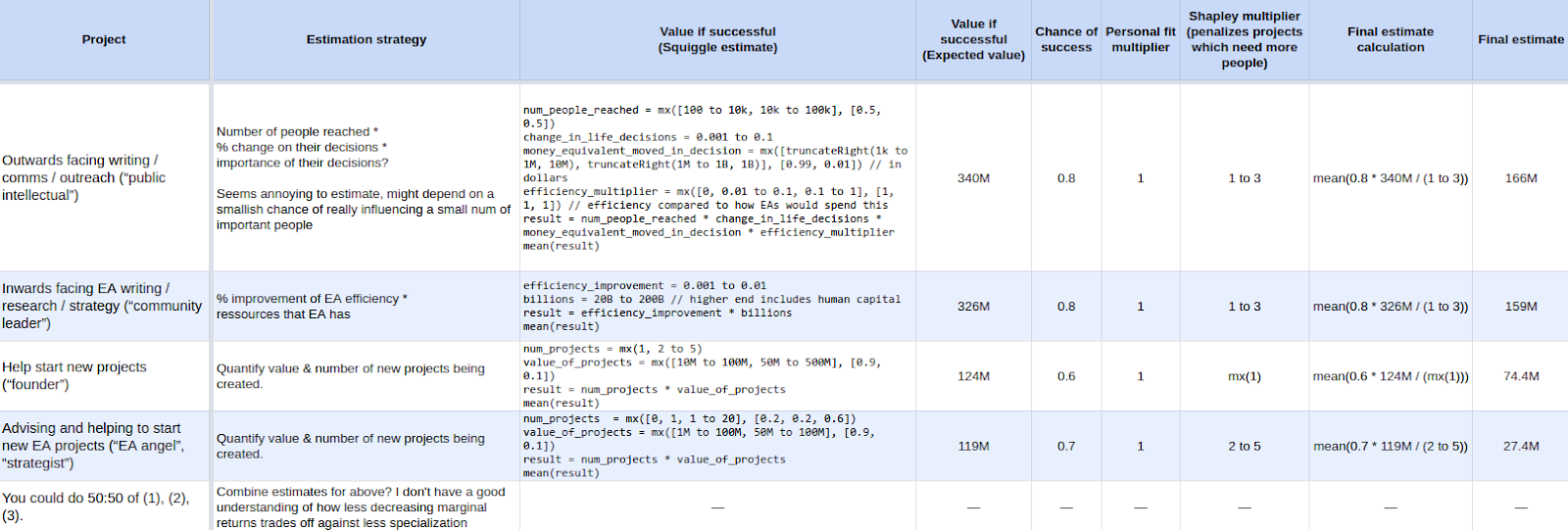
Instead of using relative values, each row estimates the value of a broad career option in dollars, i.e., in relation to how much EA should be prepared to pay for particular outcomes (e.g., the creation of 80,000 hours, or CSET). One interesting feature of dollars is that they are a pretty intuitive measure, but it breaks down a bit under interrogation (dollars in which year? adjusted for inflation? are we implicitly assuming that twice as many dollars are twice as good?). But as long as the ratios between estimates are meaningful, they are still useful for prioritization.
For a model in the above style which is more hardcore and more complex, see here (or here in the Squiggle playground.)
The estimates in this post, and overall GiveWell’s estimates of the value of AMF had been bothering me because they divide the population into very coarse chunks. This is somewhat suboptimal because the first chunk ranges from 0 to 4 years, but malaria mortality differs a fair amount between a newborn and a four-year-old.
Instead, we could express impact estimates in a more elegant functional form. I’ll sketch how this would look like, but I’ll stop halfway through because at some point the functional form would require more research about mortality at each age.
The core of the impact estimate is a function that takes the number of beneficiaries, the age distribution of a population, and the benefit of that intervention for someone of a given age, and outputs an estimate of impact.
In Squiggle, this would look as follows:
valueOfInterventionInPopulation(num_beneficiaries, population_age_distribution, benefitForPersonOfAge) = {
  age_of_beneficiaries = sampleN(population_age_distribution, num_beneficiaries)
  benefits_array = List.map(age_of_beneficiaries, {|a| benefitForPersonOfAge(a)})
  total_benefits = List.reduce(benefits_array, 0, {|acc, value| acc + value})
  total_benefits
}
So for example, if we feed the following variables to our function:
num_beneficiaries = 1000
population_age_distribution = 10 to 40
life_expectancy = 40 to 60
benefitForPersonOfAge(age) = life_expectancy - age
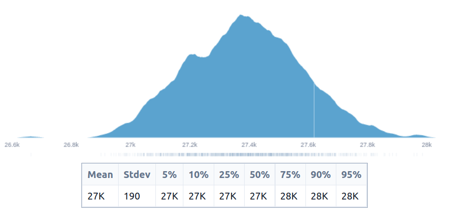
valueOfInterventionInPopulation(num_beneficiaries, population_age_distribution, benefitForPersonOfAge)Then we are saying that we are reaching 1000 people, whose age distribution looks like this:
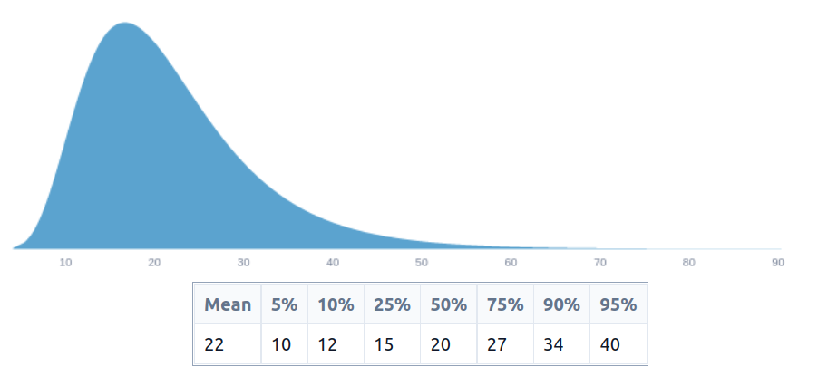
and that the benefit is just the remaining life expectancy. This produces the following estimate, in person-years:
But the assumptions we have used aren’t very realistic. We are essentially assuming that we are creating clones of people at different ages, and that they wouldn’t die until the end of their natural 40 to 50-year lifespan.
To shed these unrealistic assumptions, and produce something we can use to estimate the value of the AMF, we have to:
The first two are relatively easy to do.
For uncertainty about the number of beneficiaries, we could naïvely write:
valueWithUncertaintyAboutNumBeneficiaries(num_beneficiaries_dist, population_age_distribution, benefitForPersonOfAge) = {
  numSamples = 1000
  num_beneficiaries_samples_list = sampleN(num_beneficiaries_dist, numSamples)
  benefits_list = List.map(num_beneficiaries_samples_list, {|n| valueOfInterventionInPopulation(n, population_age_distribution, benefitForPersonOfAge)})
  result = mixture(benefits_list)
  result
}
However, that would be very slow, because we would be repeating an expensive calculation unnecessarily. Instead, we can do this:
valueWithUncertaintyAboutNumBeneficiaries(num_beneficiaries_dist, population_age_distribution, benefitForPersonOfAge) = {
  referenceN = 1000
  referenceValue = valueOfInterventionInPopulation(referenceN, population_age_distribution, benefitForPersonOfAge)

  numSamples = 1001
  num_beneficiaries_samples_list = sampleN(num_beneficiaries_dist, numSamples)
  benefits_list = List.map(num_beneficiaries_samples_list, {|n| referenceValue*n/referenceN})
  result = mixture(benefits_list)
  result
}
That is, we are calculating the value for a beneficiary population of 1000, and then we are scaling this up. This takes about 6 seconds to compute in Squiggle.
Now, when adding uncertainty about the shape of the population, we are not going to be able to use that trick, and computation will become more expensive. In the limit, maybe I would want to have a distribution of distributions. But in the meantime, I’ll just have a list of possible population shapes, and compute the shape of uncertainty over those:
valueWithUncertaintyAboutPopulationShape(num_beneficiaries_dist, population_age_distribution_list, benefitForPersonOfAge) = {
  benefits_list = List.map(population_age_distribution_list, {|population_age_distribution| valueWithUncertaintyAboutNumBeneficiaries(num_beneficiaries_dist, population_age_distribution, benefitForPersonOfAge)})
  result = mixture(benefits_list)
  result
}
population_age_distribution_list = [to(2, 40), to(2, 50), to(2, 60), to(5, 40), to(5, 50), to(5, 60), to(10, 40), to(10, 50), to(10, 60)]
We still have to tweak the benefits to better capture the benefits of distributing of malaria nets. One first attempt might look as follows:
benefitForPersonOfAge(age) = {
  result = age > 5 ? mixture(0) : {
    counterfactual_child_mortality = SampleSet.fromDist(0.01 to 0.07)
    // https://apps.who.int/gho/data/view.searo.61200?lang=en
    child_mortality_after_intervention = counterfactual_child_mortality/2
    chance_live_before = (1-(counterfactual_child_mortality))^(5-age)
    chance_live_after =   (1-(child_mortality_after_intervention))^(5-age)
    value = (chance_live_after - chance_live_before) * (life_expectancy - age)
    value
  }
  result
}
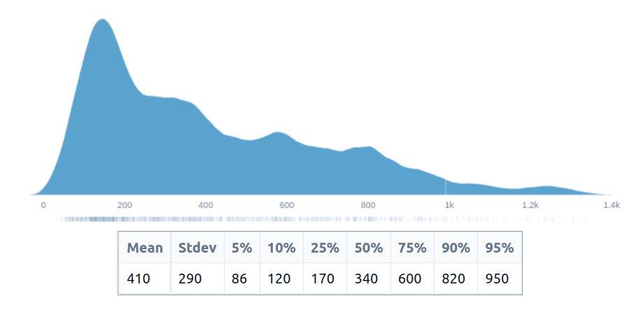
That is, we are modelling this example intervention of halving child mortality, and for child mortality to be pretty high. The final result looks like this (archived here). The output unit is years of life saved. As is, it doesn’t particularly correspond to the impact of any actual intervention, but hopefully, it could be a template that GiveWell could use, after some research.
But for reference, the distribution’s impact looks as follows:
Suppose that we have some diminishing marginal return functions. Then, we may want to estimate the optimal allocation to each opportunity.
We can express diminishing marginal returns functions using two possible syntaxes:
diminishingMarginalReturns1(funds) = 1/funds
diminishingMarginalReturns2 = {|funds| 1/(funds^2)}
The first syntax is more readable, but the second one can be used without a function definition, which is useful for manipulating functions as objects and defining them programmatically, as explained in this footnote ⤻ [1].
Once we have a few diminishing marginal return curves, we can put them in a list/array:
diminishingMarginalReturns1(funds) = 1/(100 + funds)
diminishingMarginalReturns2 = {|funds| 1/(funds^1.1)}
diminishingMarginalReturns3 = {|funds| 100/(1k + funds^1.5)}
diminishingMarginalReturns4 = {|funds| 200/(funds^2.2)}
diminishingMarginalReturns5 = {|funds| 2/(100*funds + 1)}
uselessDistribution(funds) = 0
negativeOpportunity(funds) = 0

listOfDiminishingMarginalReturns = [
  diminishingMarginalReturns1, diminishingMarginalReturns2,
  diminishingMarginalReturns3, diminishingMarginalReturns4,
  diminishingMarginalReturns5, uselessDistribution,
  negativeOpportunity, {|funds| {1/(1 + funds + funds^2)}}
]
And then we can specify our amount of funds;
availableFunds = 1M // dollars
calculationIncrement  = 1 // calculate dollar by dollar
Danger.optimalAllocationGivenDiminishingMarginalReturnsForManyFunctions(listOfDiminishingMarginalReturns, availableFunds, calculationIncrement)
So in this case, the difficulty comes not from applying a function, but from adding that function to Squiggle. This can be seen here.
Other software (e.g,. Python, R) could also do this, but the usefulness of the above comes from integrating that into Squiggle. For example, we could have an uncertain function produced by some other program, then take its mean (representing its expected value), and feed it to that calculator.
The Survival and Flourishing Fund has some software to do something like this. It has a graphical interface which people can tweak, at the expense of being a bit more simple—their diminishing marginal returns are only determined by three points
Lastly, we will define a simple toy world, which has some population growth and some economic growth, as well as some chance of extinction each year. And its value is defined as a function of the consumption of each person, times the chance that the world is still standing.
For practical purposes, after some set point we stop calculations, and we calculate the remaining value as some function of the current value. We can understand this as either a) the heat death of the universe, or b) an arbitrary limit such that we are interested in the behaviour of the system as that limit goes to infinity, but we can only extend that limit with more computation.
This setup allows us to coarsely compare an increase in consumption vs an increase in economic growth vs a reduction in existential risk. In particular, given this setup, existential risk and economic growth would be valued less than in the infinite horizon case, so if their value is greater than some increase in consumption in this toy world, we will have reason to think that this would also be the case in the real world.
The code is a bit too large to simply paste into an EA Forum post, but it can be seen here. For a further tweak, you can see leaner code here which relies on the import functionality of the squiggle-cli-experimental package.
We can also look at the impact that various interventions have on our toy world, with further details here:
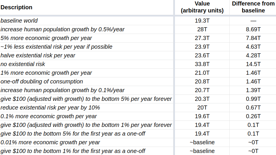
We see that of the sample interventions, increasing population growth by 0.5% has the highest impact. But 0.5%/year is a pretty large amount, and it would be pretty difficult to engineer. So further work could look at the relative difficulty of each of those interventions. Still, that table may serve to make a qualitative argument that interventions such as increasing population growth, economic growth, or reducing existential risk, are probably more valuable than directly increasing consumption.
I presented a few more advanced Squiggle models.
A running theme was that expressing estimates as functions—e.g., the chance of AGI at every point in time, the impact of an intervention for all possible ages, a list of diminishing marginal return functions for a list of interventions, a toy world with a population assigned some value at every point in time—might allow us to come up with better and more accurate estimates. Squiggle is not the only software that can do this, but hopefully it will make such estimation easier.
We can write:
listOfFunctions = [ {|funds| 1/(funds^2)}, {|funds| 1/(funds^3)}]or even
multiplyByI(i) = {|x| x*i}
listOfFunctions = List.map(List.upTo(0,10), {|i| multiplyByI(i)})
or without the need for a helper:
listOfFunctions2 = List.map(List.upTo(0,10), {|i| {|x| x*i}})
listOfFunctions2[4](2) // 4 * 2 = 8This is standard functional programming stuff, and some functionality is missing from Squiggle, such as List.length function. But still.
