Hide table of contents

Comment Permalink

I do agree that when new evidence comes in about the experts we should change how we weight them. But when we are pooling the probabilities we aren't receiving any extra evidence about the experts (?).

Right, the evidence about the experts come from the new evidence that's being updated on, not the pooling procedure. Suppose we're pooling expert judgments, and we initially consider them all equally credible, so we use a symmetric pooling method. Then some evidence comes in. Our experts update on the evidence, and we also update on how credible each expert is, and pool their updated judgments together using an asymmetric pooling method, weighting experts by how well they anticipated evidence we've seen so far. This is clearest in the case where each expert is using some model, and we believe one of their models is correct but don't know which one (the case you already agreed arithmetic averages of probabilities are appropriate). If we were weighting them all equally, and then we get some evidence that expert 1 thought was twice as likely as expert 2, then now we should think that expert 1 is twice as likely to be the one with the correct model as expert 2 is, and take a weighted arithmetic mean of their new probabilities where we weight expert 1 twice as heavily as expert 1. When you do this, your pooled probabilities handle Bayesian updates correctly. My point was that, even outside of this particular situation, we should still be taking expert credibility into account in some way, and expert credibility should depend on how well the expert anticipated observed evidence. If two experts assign odds ratios and $s_{0}$ to some event before observing new evidence, and we pool these into the odds ratio $r_{0}^{1 / 2} s_{0}^{1 / 2}$ , and then we receive some evidence causing the experts to update to $r_{1}$ and $s_{1}$ , respectively, but expert r anticipated that evidence better than expert s did, then I'd think this should mean we would weight expert r more heavily, and pool their new odds ratios into $r_{1}^{2 / 3} s_{1}^{1 / 3}$ , or something like that. But we won't handle Bayesian updates correctly if we do! The external Bayesianity property of the mean log odds pooling method means that to handle Bayesian updates correctly, we must update to the odds ratio $r_{1}^{1 / 2} s_{1}^{1 / 2}$ , as if we learned nothing about the relative credibility of the two experts.

I agree that the way I presented it I framed the extreme expert as more knowledgeable. I did this for illustrative purposes. But I believe the setting works just as well when we take both experts to be equally knowledgeable / calibrated.

I suppose one reason not to see this as unfairly biased towards mean log odds is if you generally expect experts who give more extreme probabilities to actually be more knowledgeable in practice. I gave an example in my post illustrating why this isn't always true, but a couple commenters on my post gave models for why it's true under some assumptions, and I suppose it's probably true in the data you've been using that's been empirically supporting mean log odds.

Throwing away the information from the extreme prediction seems bad.

I can see where you're coming from, but have an intuition that the geometric mean still trusts the information from outlying extreme predictions too much, which made a possible compromise solution occur to me, which to be clear, I'm not seriously endorsing.

I notice this is very surprising to me, because averaging log odds is anything but senseless.

I called it that because of its poor theoretical properties (I'm still not convinced they arise naturally in any circumstances), but in retrospect I don't really endorse this given the apparently good empirical performance of mean log odds.

log odds make Bayes rule additive, and I expect means to work well when the underlying objects are additive

My take on this is that multiplying odds ratios is indeed a natural operation that you should expect to be an appropriate thing to do in many circumstances, but that taking the nth root of an odds ratio is not a natural operation, and neither is taking geometric means of odds ratios, which combines both of those operations. On the other hand, while adding probabilities is not a natural operation, taking weighted averages of probabilities is.

My gut feeling is this argument relies on an adversarial setting where you might get exploited. And this probably means that you should come up with a probability range for the additional evidence your opponent might have.
So if you think their evidence is uniformly distributed over -1 and 1 bits, you should combine that with your evidence by adding that evidence to your logarithmic odds. This gives you a probability distribution over the possible values. Then use that spread to decide which bet odds are worth the risk of exploitation.

Right, but I was talking about doing that backwards. If you've already worked out for which odds it's worth accepting bets in each direction at, recover the probability that you must currently be assigning to the event in question. Arithmetic means of the bounds on probabilities implied by the bets you'd accept is a rough approximation to this: If you would be on X at odds implying any probability less than 2%, and you'd bet against X at odds implying any probability greater than 50%, then this is consistent with you currently assigning probability 26% to X, with a 50% chance that an adversary has evidence against X (in which case X has a 2% chance of being true), and a 50% chance that an adversary has evidence for X (in which case X has a 50% chance of being true).

I do not understand how this is about pooling different expert probabilities. But I might be misunderstanding your point.

It isn't. My post was about pooling multiple probabilities of the same event. One source of multiple probabilities of the same event is the beliefs of different experts, which your post focused on exclusively. But a different possible source of multiple probabilities of the same event is the bounds in each direction on the probability of some event implied by the betting behavior of a single expert.

See in context

Aggregating Forecasts

When pooling forecasts, use the geometric mean of odds

by Jaime Sevilla

Sep 3 202110 min read 63

125

ForecastingStatistics

Frontpage

When pooling forecasts, use the geometric mean of odds

The (extremized) geometric mean of odds empirically results in more accurate predictions

The geometric mean of odds satisfies external Bayesianity

The arithmetic mean of probabilities ignores information from extreme predictions

Do the differences between geometric mean of odds and arithmetic mean of probabilities matter in practice?

In short: There are many methods to pool forecasts. The most commonly used is the arithmetic mean of probabilities. However, there are empirical and theoretical reasons to prefer the geometric mean of the odds instead. This is particularly important when some of the predictions have extreme values. Therefore, I recommend defaulting to the geometric mean of odds to aggregate probabilities.

Epistemic status: My impression is that geometric mean of odds is the preferred pooling method among most researchers who have looked into the topic. That being said, I only cite one study with direct empirical evidence supporting my recommendation.

One key piece of advice I would give to people keen on forming better opinions of the world is to pay attention to many experts, and to reason things through a few times using different assumptions. In the context of quantitative forecasting, this results in many predictions, that together paint a more complete picture.

But, how can we aggregate the different predictions? Ideally, we would like a simple heuristic that pools the many experts and models we have considered and produce an aggregate prediction [1].

There are many possible choices for such a heuristic. A common one is to take the arithmetic mean of the individual predictions :

We see an example of this approach in this article from Luisa Rodriguez, where it is used to aggregate some predictions about the chances of a nuclear war in a year.

A different heuristic, which I will argue in favor of, is to take the geometric mean of the odds:

o = \sqrt[N]{o_{1} \times \dots \times o_{N}}

Whereas the arithmetic mean adds the values together and divides by the number of values, the geometric mean multiplies all the values and then takes the N-th root of the product (where N = number of values).

And the odds equal the probability of an event divided by its complement, $o = p / (1 - p)$ .[2]

For example, in Rodriguez's article we have four predictions from different sources [3]:

Probabilities	Odds
1.40%	1:70
2.21%	1:44
0.39%	1:255
0.40%	1:249

Rodriguez takes as an aggregate the arithmetic mean of the probabilities $[1.40 % + 2.21 % + 0.39 % + 0.40 %] / 4 = 1.10 %$ , which corresponds to pooled odds of about $1 : 91$ .
If we take the geometric mean of the odds instead we will end with pooled odds of $(1 : 70 \cdot 1 : 44 \cdot 1 : 255 \cdot 1 : 249)^{1 / 4} \approx 1 : 118$ , which corresponds to a pooled probability of about $0.84 %$ .

In the remainder of the article I will argue that the geometric mean of odds is both empirically more accurate and has some compelling theoretical properties. In practice, I believe we should largely prefer to aggregate probabilities using the geometric mean of odds.

The (extremized) geometric mean of odds empirically results in more accurate predictions

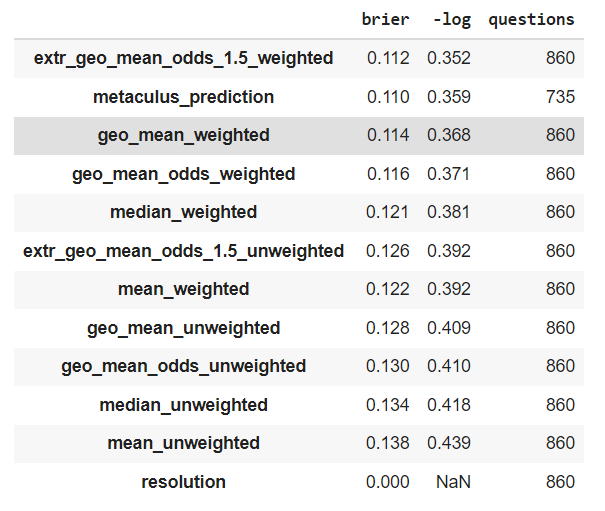
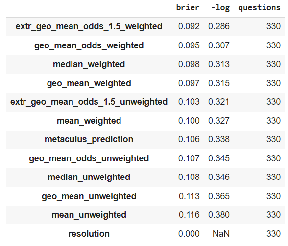
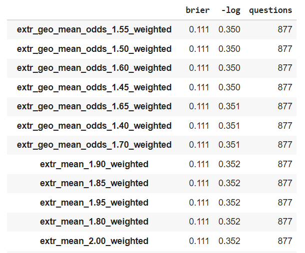
(Satopää et al, 2014) empirically explores different aggregation methods, including average probabilities, the median probability, and the geometric mean of the odds - as well as some more complex methods of aggregating forecasts like and extremized version of the geometric mean of the odds and the beta transformed linear opinion pool. They aggregate responses from 1300 forecasters over 69 questions on geopolitics [4].

In summary, they find that the extremized geometric mean of odds performs best in terms of the Brier score of its predictions. The non-extremized geometric mean of odds robustly outperforms the arithmetic mean of probabilities and the median, though it performs worse than some of the more complex methods.

We haven't quite explained what extremizing is, but it involves raising the pooled odds to a power $a > 1$ [5]:

o = {(\sqrt[N]{o_{1} \times \dots \times o_{N}})}^{a}

In their dataset, the extremizing parameter $a$ that attains the best Brier score falls between $1.161$ and $3.921$ . As a handy heuristic, when extremizing I suggest using a power of $2.5$ in practice. My intuition is that extremizing makes most sense when aggregating data from underconfident experts, and I would not use it when aggregating personal predictions derived from different approaches. This is because extremizing is meant to be a correction for forecaster underconfidence [6]. That being said, it is unclear to me when extremizing helps (eg see Simon_M's comment for an example where extremizing does not help improve the aggregate predictions).

What do other experiments comparing different pooling methods find? (Seaver, 1978) performs an experiment where the performance of the arithmetic mean of probabilities and the geometric mean of odds is similar (he studies 11 groups of 4 people each, on 100 general trivia questions). However, Seaver studies questions where the individual probabilities are in a range between 5% and 95%, where the difference between the two methods is small.

In my superficial exploration of the literature I haven't been able to find many more empirical studies (EDIT: see Simon_M's comment here for a comparison of pooling methods on Metaculus questions). There are plenty of simulation studies - for example (Allard et al, 2012) find better performance of the geometric mean of odds in simulations.

The geometric mean of odds satisfies external Bayesianity

(Allard et al, 2012) explore the theoretical properties of several aggregation methods, including the geometric average of odds.

They speak favorably of the geometric mean of odds, mainly because it is the only pooling method that satisfies external Bayesianity [7] This result was proved before in (Genest, 1984).

External Bayesianity means that if the experts all agree on the strength of the Bayesian updates of each available piece of evidence, it does not matter whether they aggregate their posteriors, or if they aggregate their priors first then apply the updates - the result is the same.

External Bayesianity is compelling because it means that, from the outside, the group of experts behaves like a Bayesian agent - it has a consistent set of priors that are updated according to Bayes rule.

For more discussion on external Bayesianity, see (Madanski, 1964).

While suggestive, I consider external Bayesianity a weaker argument than the empirical study of (Satopää et al, 2014). This is because the arithmetic mean of probabilities also has some good theoretical properties of its own, and it is unclear which properties are most important. I do however believe that external Bayesianity is more compelling than the other properties I have seen discussed in the literature [8].

The arithmetic mean of probabilities ignores information from extreme predictions

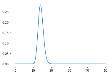
The arithmetic mean of probabilities ignores extreme predictions in favor of tamer results, to the extent that even large changes to individual predictions will barely be reflected in the aggregate prediction.

As an illustrative example, consider an outsider expert and an insider expert on a topic, who are eliciting predictions about an event. The outsider expert is reasonably uncertain about the event, and each of them assigns a probability of around 10% to the event. The insider has priviledged information about the event, and assigns to it a very low probability.

Ideally, we would like the aggregate probability to be reasonably sensitive to the strength of the evidence provided by the insider expert - if the insider assigns a probability of 1 in 1000 the outcome should be meaningfully different than if the insider assigns a probability of 1 in 10,000 [9].

The arithmetic mean of probabilities does not achieve this - in both cases the pooled probability is around $(10 % + 1 / 1, 000) / 2 \approx (10 % + 1 / 10, 000) / 2 \approx 5.00 %$ . The uncertain prediction has effectively overwritten the information in the more precise prediction.

The geometric mean of odds works better in this situation. We have that $[(1 : 9) \times (1 : 999)]^{1 / 2} \approx 1 : 95$ , while $[(1 : 9) \times (1 : 9999)]^{1 / 2} \approx 1 : 300$ . Those correspond respectively to probabilities of 1.04% and 0.33% - showing the greater sensitivity to the evidence the insider brings to the table.

See (Baron et al, 2014) for more discussion on the distortive effects of the arithmetic mean of probabilities and other aggregates.

Do the differences between geometric mean of odds and arithmetic mean of probabilities matter in practice?

Not often, but often enough. For example, we already saw that the geometric mean of odds outperforms all other simple methods in (Satopää et al, 2014), yet they perform similarly in (Seaver, 1978).

Indeed, the difference between one method or another in particular examples may be small. Case in point, the nuclear war example - the difference between the geometric mean of odds and arithmetic mean of probabilities was less than 3 in 1,000.

This is often the case. If the individual probabilities are in the 10% to 90% range, then the absolute difference in aggregated probabilities between these two methods will typically fall in the 0% to 3% range.

Though, even if the difference in probabilities is not large, the difference in odds might still be significant. In the nuclear war example above there was a factor of 1.3 between the odds implied by both methods. Depending on the application this might be important [10].

Furthermore, the choice of aggregation method starts making more of a difference as your probabilities become more extreme : if the individual probabilities are within the range 0.7% to 99.2% then the difference will typically fall between 0% to 18% [11].

Conclusion

If you face a situation where you have to pool together some predictions, use the geometric mean of odds. Compared to the arithmetic mean of probabilities, the geometric mean of odds is similarly complex*, one empirical study and many simulation studies found that it results in more accurate predictions, and it satisfies some appealing theoretical properties, like external Bayesianity and not overweighting uncertain predictions.

* Provided you are willing to to work with odds instead of probabilities, which you might not be comfortable with.

Acknowledgements

Ben Snodin helped me with detailed discussion and feedback, which helped me clarify my intuitions about the topic while we discussed some examples. Without his help I would have written a much poorer article.

I previously wrote about this topic on LessWrong, where UnexpectedValues and Nuño Sempere helped me clarify a few details I had wrong.

Spencer Greenberg wrote a Facebook post about aggregating forecasts that spurred discussion on the topic. I am particularly grateful to Spencer Greenberg, Gustavo Lacerda and Guy Srinivasan for their thoughts.

And thank you Luisa Rodriguez for the excellent post on nuclear war. Sorry for picking on your aggregation in the example!

Footnotes

[1] We will focus on prediction of binary events, summarized as a single number $p$ , the probability of the event. Prediction for multiple outcome events and continuous distributions fall outside of the scope of this post, though equivalent concepts to the geometric average of odds exist for those cases. For example, for multiple outcome events we may use the geometric mean of the vector odds, and for continuous distributions we may use $\prod_{i = 1}^{N} f_{i}^{1 / N} / \int \prod_{i = 1}^{N} f_{i}^{1 / N}$ as in (Genest, 1984).

[2] There are many equivalent formulations for the formula of geometric mean odds pooling in terms of probabilities .

One possibility is

p = \frac{\prod_{i = 1}^{N} p_{i}^{1 / N}}{\prod_{i = 1}^{N} p_{i}^{1 / N} + \prod_{i = 1}^{N} (1 - p_{i})^{1 / N}}

That is, the pooled probability equals the geometric mean of the probabilities divided by the sum of the geometric mean of the probabilities and the geometric mean of the complementary probabilities.

Another possibile expression for the resulting pooled probability is:

p = \frac{\prod_{i = 1}^{n} {\frac{p_{i}}{1 - p_{i}}}^{1 / N}}{1 + \prod_{i = 1}^{n} {\frac{p_{i}}{1 - p_{i}}}^{1 / N}}

[3] I used this calculator to compute nice approximations of the odds.

[4] (Satopää et al, 2014) also study simulations in their paper. The results of their simulations are similar to their empirical results.

[5] The method is hardly innovative - many others have proposed similar corrections to pooled aggregates, with similar proposals appearing as far back as (Karmarkar, 1978).

[6] Why use extremizing in the first place?

(Satopää et al, 2014) derive this correction from assuming that the predictions of the experts are individually underconfident, and need to be pushed towards an extreme. (Baron et al, 2014) derive the same correction from a toy scenario in which each forecaster regresses their forecast towards uncertainty, by assuming that calibrated forecasts tend to be distributed around 0.

Despite the wide usage of extremizing, I haven't yet read a theoretical justification for extremizing that fully convinces me. It does seem to get better results in practice, but there is a risk this is just overfitting from the choice of the extremizing parameter.

Because of this, I am more hesitant to outright recommend extremizing.

[7] Technically, any weighted geometric average of the odds satisfies external Bayesianity. Concretely, the family of aggregation methods according to the formula:

o = N \prod i = 1 o_{i}^{w_{i}}

where $w_{i} > 0$ and $\sum_{i = 1}^{N} w_{i} = 1$ covers all externally Bayesian methods. Among them, the only one that does not privilege any of the experts is of course the traditional geometric average of odds where $w_{i} = 1 / N$ .

[8] The most discussed property of the arithmetic mean of probabilities is marginalization. We say that a pooling method respects marginalization if the marginal distribution of the pooled probabilities equals the pooled distribution of the marginals.

There is some discussion on marginalization in (Lindley, 1983), where the author argues that it is a flawed concept. More discussion and a summary of Lindley's results can be found here.

[9] There are some concievable scenarios where we might not want this behaviour. For example, if we are risk averse in a way such that we prefer to defer to the most uncertain experts, or if we expect the predictions to be noisy, and thus we would like to avoid outliers. But largely I think those are uncommon and somewhat contrived situations.

[10] The difference between the methods is probably not significant when using the aggregate in a cost-benefit analysis, since expected value depends linearly on the probability which does not change much. But it is probably significant when using the aggregate as a base-rate for further analysis, since the posterior odds depend linearly on the prior odds, which change moderately.

[11] To compute the ranges I took 100,000 samples of 10 probabilities whose log-odd expression was normally distributed and reported the 5% and 95% quantiles for both the individual probabilities sampled and the difference between the pooled probabilities implied by both methods on each sample. Here is the code I used to compute these results.

Bibliography

Allard, D., A. Comunian, and P. Renard. 2012. ‘Probability Aggregation Methods in Geoscience’. Mathematical Geosciences 44 (5): 545–81. https://doi.org/10.1007/s11004-012-9396-3.

Baron, Jonathan, Barb Mellers, Philip Tetlock, Eric Stone, and Lyle Ungar. 2014. ‘Two Reasons to Make Aggregated Probability Forecasts More Extreme’. Decision Analysis 11 (June): 133–45. https://doi.org/10.1287/deca.2014.0293.

Genest, Christian. 1984. ‘A Characterization Theorem for Externally Bayesian Groups’. The Annals of Statistics 12 (3): 1100–1105.

Lindley, Dennis. 1983. ‘Reconciliation of Probability Distributions’. Operations Research 31 (5): 866–80.

Karmarkar, Uday S. 1978. ‘Subjectively Weighted Utility: A Descriptive Extension of the Expected Utility Model’. Organizational Behavior and Human Performance 21 (1): 61–72. https://doi.org/10.1016/0030-5073(78)90039-9.

Madansky, Albert. 1964. ‘Externally Bayesian Groups’. RAND Corporation. https://www.rand.org/pubs/research_memoranda/RM4141.html.

Satopää, Ville A., Jonathan Baron, Dean P. Foster, Barbara A. Mellers, Philip E. Tetlock, and Lyle H. Ungar. 2014. ‘Combining Multiple Probability Predictions Using a Simple Logit Model’. International Journal of Forecasting 30 (2): 344–56. https://doi.org/10.1016/j.ijforecast.2013.09.009.

Seaver, David Arden. 1978. ‘Assessing Probability with Multiple Individuals: Group Interaction Versus Mathematical Aggregation.’ DECISIONS AND DESIGNS INC MCLEAN VA. https://apps.dtic.mil/sti/citations/ADA073363.

125 Reactions

My current best guess on how to aggregate forecasts

19 comments39 karma

Mentioned in

175Samotsvety's AI risk forecasts

155Samotsvety Nuclear Risk Forecasts — March 2022

123Forecasts estimate limited cultured meat production through 2050

120Update to Samotsvety AGI timelines

111‘Dissolving’ AI Risk – Parameter Uncertainty in AI Future Forecasting

Load more (5/22)

Comments63

Sorted by

New & upvoted

Click to highlight new comments since: Today at 11:17 AM

Simon_MSep 3 202154

tl;dr The conclusions of this article hold up in an empirical test with Metaculus data

Looking at resolved binary Metaculus questions and using 5 different methods to pool the community estimate.

Geometric mean of probabilities
Geometric mean of odds / Arithmetic mean of log-odds
Median of odds (current Metaculus forecast)
Arithmetic mean of odds
Proprietary Metaculus forecast

Also looking at two different scoring rules (Brier and Log) I find rankings as (smaller is better in my table):

Metaculus prediction is currently the best[2]
Geometric mean of probabilities
Geometric mean of odds / Arithmetic mean of log-odds
Median
Arithmetic mean of probabilities

Another conclusion which follows from this is that weighting is much more important than how you aggregate your probabilities. Roughly speaking:

Weighting by quality of predictor beats...
Weighting by how recently they updated beats...
No weighting at all

(I also did this analysis for both weighted[1] and unweighted odds)

	brier	-log	questions
metaculus_prediction	0.110	0.359	722
geo_mean_weighted	0.114	0.368	847
geo_mean_odds_weighted	0.116	0.370	847
median_weighted	0.121	0.380	847
extr_geo_mean_odds_2.5_weighted	0.115	0.386	847
mean_weighted	0.122	0.392	847
geo_mean_unweighted	0.128	0.409	847
geo_mean_odds_unweighted	0.130	0.409	847
median_unweighted	0.134	0.417	847
extr_geo_mean_odds_2.5_unweighted	0.131	0.430	847
mean_unweighted	0.138	0.438	847

(Analysis on ~850 questions, predictors per question: [ 34 , 51 , 78 , 122, 188] (10th, 25th, 50th, 75th, 90th percentile)

[1] Metaculus weights it's predictions by recency:

Each predicting player is marked with a number (starting at 1) that orders them from oldest active prediction to newest prediction. The individual predictions are given weights $w (n) \propto e^{\sqrt{n}}$ and combined to form a weighted community distribution function.

[2] This doesn't actually hold up more recently, where the Metaculus prediction has been underperforming.

Jaime SevillaSep 4 20216

META: Do you think you could edit this comment to include...

The number of questions, and aggregated predictions per question?
The information on extremized geometric mean you computed below (I think it is not receiving as much attention due to being buried in the replies)?
Possibly a code snippet to reproduce the results?

Thanks in advance!

Simon_MSep 8 202118

import requests, json
import numpy as np
import pandas as pd

def fetch_results_data():
    response = {"next":"https://www.metaculus.com/api2/questions/?limit=100&status=resolved"}

    results = []
    while response["next"] is not None:
        print(response["next"])
        response = json.loads(requests.get(response["next"]).text)
        results.append(response["results"])
    return sum(results,[])


all_results = fetch_results_data()
binary_qns = [q for q in all_results if q['possibilities']['type'] == 'binary' and q['resolution'] in [0,1]]
binary_qns.sort(key=lambda q: q['resolve_time'])

def get_estimates(ys):
    xs = np.linspace(0.01, 0.99, 99)
    odds = xs/(1-xs)
    mean = np.sum(xs * ys) / np.sum(ys)
    geo_mean = np.exp(np.sum(np.log(xs) * ys) / np.sum(ys))
    geo_mean_odds = np.exp(np.sum(np.log(odds) * ys) / np.sum(ys))
    geo_mean_odds_p = geo_mean_odds/(1+geo_mean_odds)
    extremized_odds = np.exp(np.sum(2.5 * np.log(odds) * ys) / np.sum(ys))
    extr_geo_mean_odds = extremized_odds/(1+extremized_odds)
    median = weighted_quantile(xs, 0.5, sample_weight=ys)
    return [mean, geo_mean, median, geo_mean_odds_p, extr_geo_mean_odds], ["mean", "geo_mean", "median", "geo_mean_odds", "extr_geo_mean_odds_2.5"]

def brier(p, r):
    return (p-r)**2
def log_s(p, r):
    return -(r * np.log(p) + (1-r)*np.log(1-p))

X = []

for q in binary_qns:
    weighted = q['community_prediction']['full']['y']
    unweighted = q['community_prediction']['unweighted']['y']
    t = [q['resolution'], q["community_prediction"]["history"][-1]["nu"]]
    all_names = ['resolution', 'users']
    for (e, ys) in [('_weighted', weighted), ('_unweighted', unweighted)]:
        s, names = get_estimates(np.array(ys))
        all_names += [n+e for n in names]
        t += s
    t += [q["metaculus_prediction"]["full"]]
    all_names.append("metaculus_prediction")
    X.append(t)
df = pd.DataFrame(X, columns=all_names)

df_v = df[:]

pd.concat([df_v.apply(lambda x: brier(x, df["resolution"]), axis=0).mean().to_frame("brier"),
           (df_v.apply(lambda x: log_s(x, df["resolution"]), axis=0)).mean().to_frame("-log"),
           df_v.count().to_frame("questions"),
          ], axis=1).sort_values('-log')[:-1].round(3)

Vasco Grilo🔸Feb 6 20242

Thanks for the analysis, Simon!

I think it would be valuable to repeat it specifically for questions where there is large variance across predictions, where the choice of the aggregation method is specially relevant. Under these conditions, I suspect methods like the median or geometric mean will be even better than methods like the mean because the latter ignore information from extremely low predictions, and overweight outliers.

MaxRaSep 3 20213

Cool, that’s really useful to know. Can you also check how extremizing the odds with different parameters performs?

Simon_MSep 3 202112

	brier	-log
metaculus_prediction	0.110	0.360
geo_mean_weighted	0.115	0.369
extr_geo_mean_odds_2.5_weighted	0.116	0.387
geo_mean_odds_weighted	0.117	0.371
median_weighted	0.121	0.381
mean_weighted	0.122	0.393
geo_mean_unweighted	0.128	0.409
geo_mean_odds_unweighted	0.130	0.410
extr_geo_mean_odds_2.5_unweighted	0.131	0.431
median_unweighted	0.134	0.417
mean_unweighted	0.138	0.439

Jaime SevillaSep 3 20214

Thank you for the superb analysis!

This increases my confidence in the geo mean of the odds, and decreases my confidence in the extremization bit.

I find it very interesting that the extremized version was consistently below by a narrow margin. I wonder if this means that there is a subset of questions where it works well, and another where it underperforms.

One question / nitpick: what do you mean by geometric mean of the probabilities? If you just take the geometric mean of probabilities then you do not get a valid probability - the sum of the pooled ps and (1-p)s does not equal 1. You need to rescale them, at which point you end with the geometric mean of odds.

Unexpected values explains this better than me here.

Simon_MSep 3 20215

I find it very interesting that the extremized version was consistently below by a narrow margin. I wonder if this means that there is a subset of questions where it works well, and another where it underperforms.

I think it's actually that historically the Metaculus community was underconfident (see track record here before 2020 vs after 2020).

Extremizing fixes that underconfidence, but also the average predictor improving their ability also fixed that underconfidence.

One question / nitpick: what do you mean by geometric mean of the probabilities?

~~Metaculus has a known bias towards questions resolving positive~~ . Metaculus users have a known bias overestimating the probabilities of questions resolving positive. (Again - see the track record). Taking a geometric median of the probabilities of the events happening will give a number between 0 and 1. (That is, a valid probability). It will be inconsistent with the estimate you'd get if you flipped the question HOWEVER Metaculus users also seem to be inconsistent in that way, so I thought it was a neat way to attempt to fix that bias. I should have made it more explicit, that's fair.

Edit: Updated for clarity based on comments below

Jaime SevillaSep 3 20211

but also the average predictor improving their ability also fixed that underconfidence

What do mean by this?

Metaculus has a known bias towards questions resolving positive

Oh I see!

It is very cool that this works.

One thing that confuses me - when you take the geometric mean of probabilities you end up with . So the pooled probability gets slighly nudged towards 0 in comparison to what you would get with the geometric mean of odds. Doesn't that mean that it should be less accurate, given the bias towards questions resolving positively?

What am I missing?

Simon_MSep 3 20212

but also the average predictor improving their ability also fixed that underconfidence
What do mean by this?

I mean in the past people were underconfident (so extremizing would make their predictions better). Since then they've stopped being underconfident. My assumption is that this is because the average predictor is now more skilled or because more predictors improves the quality of the average.

Doesn't that mean that it should be less accurate, given the bias towards questions resolving positively?

The bias isn't that more questions resolve positively than users expect. The bias is that users expect more questions to resolve positive than actually resolve positive. Shifting probabilities lower fixes this.

Basically lots of questions on Metaculus are "Will X happen?" where X is some interesting event people are talking about, but the base rate is perhaps low. People tend to overestimate the probability of X relative to what actually occurs.

NunoSempereSep 3 20213

The bias isn't that more questions resolve positively than users expect. The bias is that users expect more questions to resolve positive than actually resolve positive.

I don't get what the difference between these is.

Simon_MSep 3 20214

"more questions resolve positively than users expect"

Users expect 50 to resolve positively, but actually 60 resolve positive.

"users expect more questions to resolve positive than actually resolve positive"

Users expect 50 to resolve positive, but actually 40 resolve positive.

I have now editted the original comment to be clearer?

NunoSempereSep 6 20212

Cheers

Jaime SevillaSep 3 20211

I mean in the past people were underconfident (so extremizing would make their predictions better). Since then they've stopped being underconfident. My assumption is that this is because the average predictor is now more skilled or because more predictors improves the quality of the average.

Gotcha!

The bias isn't that more questions resolve positively than users expect.

Oh I see!

Jaime SevillaSep 3 20212

(I note these scores are very different than in the first table; I assume these were meant to be the Brier scores instead?)

[This comment is no longer endorsed by its author]Reply

Simon_MSep 3 20212

Yes - copy and paste fail - now corrected

Jaime SevillaOct 6 20211

I was curious about why the extremized geo mean of odds didn't seem to beat other methods. Eric Neyman suggested trying a smaller extremization factor, so I did that.

I tried an extremizing factor of 1.5, and reused your script to score the performance on recent binary questions. The result is that the extremized prediction comes on top.

This has restored my faith on extremization. On hindsight, recommending a fixed extremization factor was silly, since the correct extremization factor is going to depend on the predictors being aggregated and the topics they are talking about.

Going forward I would recommend people who want to apply extremization to study what extremization factors would have made sense in past questions from the same community.

I talk more about this in my new post.

Simon_MOct 6 202110

This has restored my faith on extremization

I think this is the wrong way to look at this.

Metaculus was way underconfident originally. (Prior to 2020, 22% using their metric). Recently it has been much better calibrated - (2020- now, 4% using their metric).

Of course if they are underconfident then extremizing will improve the forecast, but the question is what is most predictive going forward. Given that before 2020 they were 22% underconfident, more recently 4% underconfident, it seems foolhardy to expect them to be underconfident going forward.

I would NOT advocate extremizing the Metaculus community prediction going forward.

More than this, you will ALWAYS be able to find an extremize parameter which will improve the forecasts unless they are perfectly calibrated. This will give you better predictions in hindsight but not better predictions going forward. If you have a reason to expect forecasts to be underconfident, by all means extremize them, but I think that's a strong claim which requires strong evidence.

Jaime SevillaOct 6 20211

I get what you are saying, and I also harbor doubts about whether extremization is just pure hindsight bias or if there is something else to it.

Overall I still think its probably justified in cases like Metaculus to extremize based on the extremization factor that would optimize the last 100 resolved questions, and I would expect the extremized geo mean with such a factor to outperform the unextremized geo mean in the next 100 binary questions to resolve (if pressed to put a number on it maybe ~70% confidence without thinking too much).

My reasoning here is something like:

There seems to be a long tradition of extremizing in the academic literature (see the reference in the post above). Though on the other hand empirical studies have been sparse, and eg Satopaa et al are cheating by choosing the extremization factor with the benefit of hindsight.
In this case I didn't try too hard to find an extremization factor that would work, just two attempts. I didn't need to mine for a factor that would work. But obviously we cannot generalize from just one example.
Extremizing has an intuitive meaning as accounting for the different pieces of information across experts that gives it weight (pun not intended). On the other hand, every extra parameter in the aggregation is a chance to shoot off our own foot.
Intuitively it seems like the overall confidence of a community should be roughly continuous over time? So the level of underconfidence in recent questions should be a good indicator of its confidence for the next few questions.

So overall I am not super convinced, and a big part of my argument is an appeal to authority.

Also, it seems to be the case that extremization by 1.5 also works when looking at the last 330 questions.

I'd be curious about your thoughts here. Do you think that a 1.5-extremized geo mean will outperform the unextremized geo mean in the next 100 questions? What if we choose a finetuned extremization factor that would optimize the last 100?

Simon_MOct 7 20216

Looking at the rolling performance of your method (optimize on last 100 and use that to predict), median and geo mean odds, I find they have been ~indistinguishable over the last ~200 questions. If I look at the exact numbers, extremized_last_100 does win marginally, but looking at that chart I'd have a hard time saying "there's a 70% chance it wins over the next 100 questions". If you're interested in betting at 70% odds I'd be interested.

There seems to be a long tradition of extremizing in the academic literature (see the reference in the post above). Though on the other hand empirical studies have been sparse, and eg Satopaa et al are cheating by choosing the extremization factor with the benefit of hindsight.

No offense, but the academic literature can do one.

In this case I didn't try too hard to find an extremization factor that would work, just two attempts. I didn't need to mine for a factor that would work. But obviously we cannot generalize from just one example.

Again, I don't find this very persuasive, given what I already knew about the history of Metaculus' underconfidence.

Extremizing has an intuitive meaning as accounting for the different pieces of information across experts that gives it weight (pun not intended). On the other hand, every extra parameter in the aggregation is a chance to shoot off our own foot.

I think extremizing might make sense if the other forecasts aren't public. (Since then the forecasts might be slightly more independent). When the other forecasts are public, I think extremizing makes less sense. This goes doubly so when the forecasts are coming from a betting market.

Intuitively it seems like the overall confidence of a community should be roughly continuous over time? So the level of underconfidence in recent questions should be a good indicator of its confidence for the next few questions.

I find this the most persuasive. I think it ultimately depends how you think people adjust for their past calibration. It's taken the community ~5 years to reduce it's under-confidence, so maybe it'll take another 5 years. If people immediately update, I would expect this to be very unpredictable.

Eric NeymanSep 4 202129

Thanks for writing this up; I agree with your conclusions.

There's a neat one-to-one correspondence between proper scoring rules and probabilistic opinion pooling methods satisfying certain axioms, and this correspondence maps Brier's quadratic scoring rule to arithmetic pooling (averaging probabilities) and the log scoring rule to logarithmic pooling (geometric mean of odds). I'll illustrate the correspondence with an example.

Let's say you have two experts: one says 10% and one says 50%. You see these predictions and need to come up with your own prediction, and you'll be scored using the Brier loss: (1 - x)^2, where x is the probability you assign to whichever outcome ends up happening (you want to minimize this). Suppose you know nothing about pooling; one really basic thing you can do is to pick an expert to trust at random: report 10% with probability 1/2 and 50% with probability 1/2. Your expected Brier loss in the case of YES is (0.81 + 0.25)/2 = 0.53, and your expected loss in the case of NO is (0.01 + 0.25)/2 = 0.13.

But, you can do better. Suppose you say 35% -- then your loss is 0.4225 in the case of YES and 0.1225 in the case of NO -- better in both cases! So you might ask: what is the strategy the gives me the largest possible guaranteed improvement over choosing a random expert? The answer is linear pooling (averaging the experts). This gets you 0.49 in the case of YES and 0.09 in the case of NO (an improvement of 0.04 in each case).

Now suppose you were instead being scored with a log loss -- so your loss is -ln(x), where x is the probability you assign to whichever outcome ends up happening. Your expected log loss in the case of YES is (-ln(0.1) - ln(0.5))/2 ~ 1.498, and in the case of NO is (-ln(0.9) - ln(0.5))/2 ~ 0.399.

Again you can ask: what is the strategy that gives you the largest possible guaranteed improvement of this "choose a random expert" strategy? This time, the answer is logarithmic pooling (taking the geometric mean of the odds). This is 25%, which has a loss of 1.386 in the case of YES and 0.288 in the case of NO, an improvement of about 0.111 in each case.

(This works just as well with weights: say you trust one expert more than the other. You could choose an expert at random in proportion to these weights; the strategy that guarantees the largest improvement over this is to take the weighted pool of the experts' probabilities.)

This generalizes to other scoring rules as well. I co-wrote a paper about this, which you can find here, or here's a talk if you prefer.

What's the moral here? I wouldn't say that it's "use arithmetic pooling if you're being scored with the Brier score and logarithmic pooling if you're being scored with the log score"; as Simon's data somewhat convincingly demonstrated (and as I think I would have predicted), logarithmic pooling works better regardless of the scoring rule.

Instead I would say: the same judgments that would influence your decision about which scoring rule to use should also influence your decision about which pooling method to use. The log scoring rule is useful for distinguishing between extreme probabilities; it treats 0.01% as substantially different from 1%. Logarithmic pooling does the same thing: the pool of 1% and 50% is about 10%, and the pool of 0.01% and 50% is about 1%. By contrast, if you don't care about the difference between 0.01% and 1% ("they both round to zero"), perhaps you should use the quadratic scoring rule; and if you're already not taking distinctions between low and extremely low probabilities seriously, you might as well use linear pooling.

Peter WildefordOct 22 202116

I want to add a little explainer here on how to actually calculate the geometric mean of odds. At least I'm pretty sure how this works - please correct my math if I am not right!

Say you have four forecasts given in probabilities: 10%, 30%, 40%, and 90%.

First you must convert to odds using o = p/(1-p)

O1 = 0.1/(1-0.1) = 0.111111111 O2 = 0.3/(1-0.3) = 0.428571429 O3 = 0.4/(1-0.4) = 0.666666667 O4 = 0.9/(1-0.9) = 9

Now that you have odds, use the geometric mean. The geometric mean is the nth root of the product of n numbers.

geomean(O1, O2, O3, O4) = 4th root of O1 * O2 * O3 * O4 = 4th root of 0.111111111 * 0.428571429 * 0.666666667 * 9 = 4th root of 0.285714286 = 0.731110446

Now, if you're like me, it is easier to think with probabilities instead of odds, so you will want to transform it back. This is done using p = o/(o+1).

p = o / (o + 1) p = 0.731110446 / (0.731110446 + 1) = ~42%

Note that this result (~42%) is different from the geometric mean of probabilities (~32%) and different from the mean of probabilities (~43%).

SiebeRozendalSep 7 202114

Interesting! Seems intuitively right.

I wonder though: how would this affect expected value calculations? Doesn't this have far-reaching consequences?

One thing I have always wondered about is how to aggregate predicted values that differ by orders of magnitude. E.g. person A's best guess is that the value of x will be 10, person B's guess is that it will be 10,000. Saying that the expected value of x is ~5,000 seems to lose a lot of information. For simple monetary betting, this seems fine. For complicated decision-making, I'm less sure.

Jaime SevillaSep 8 202120

Let's work this example through together! (but I will change the quantities to 10 and 20 for numerical stability reasons)

One thing we need to be careful with is not mixing the implied beliefs with the object level claims.

In this case, person A's claim that the value is is more accurately a claim that the beliefs of person A can be summed up as some distribution over the positive numbers, eg a log normal with parameters $μ_{A} = log m_{A}$ and $σ_{A}$ . So the density distribution of beliefs of A is $f_{A} = \frac{1}{x σ_{A} \sqrt{2 π}} exp [- \frac{(ln x - μ_{A})^{2}}{2 σ_{A}^{2}}]$ (and similar for person B, with $m_{B} = 20$ ). The scale parameters $σ_{A}, σ_{B}$ intuitively represent the uncertainty of person A and person B.

Taking $σ_{A} = σ_{B} = 0.1$ , these densities look like:

Note that the mean of these distributions is slightly displaced upwards from the median $exp μ$ . Concretely, the mean is computed as $exp [μ + \frac{σ^{2}}{2}]$ , and equals 10.05 and 20.10 for person A and person B respectively.

To aggregate the distributions, we can use the generalization of the geometric mean of odds referred to in footnote [1] of the post.

According to that, the aggregated distribution has a density $f = \frac{{\sqrt{f}}_{A} \cdot {\sqrt{f}}_{B}}{\int {\sqrt{f}}_{A} \cdot {\sqrt{f}}_{B}}$ .

The plot of the aggregated density looks like:

I actually notice that I am very surprised about this - I expected the aggregate distribution to be bimodal, but here it seems to have a single peak.

For this particular example, a numerical approximation of the expected value seems to equal around 14.21 - which exactly equals the geometric mean of the means.

I am not taking away any solid conclusions from this exercise - I notice I am still very confused about how the aggregated distribution looks like, and I encountered serious numerical stability issues when changing the parameters, which make me suspect a bug.

Maybe a Monte Carlo approach for estimating the expected value would solve the stability issues - I'll see if I can get around to that at some point.

Meanwhile, here is my code for the results above.

EDIT: Diego Chicharro has pointed out to me that the expected value can be easily computed analytically in Mathematica.

The resulting expected value of the aggregated distribution is $exp [\frac{μ_{A} σ_{B}^{2} + μ_{B} σ_{A}^{2} + σ_{A}^{2} σ_{B}^{2}}{σ_{A}^{2} + σ_{B}^{2}}]$ .

In the case where $σ_{A}^{2} = σ_{B}^{2} = σ^{2}$ we have then that the expected value is $exp [\frac{μ_{A} σ^{2} + μ_{B} σ^{2} + σ^{2} σ^{2}}{σ^{2} + σ^{2}}] = exp [\frac{μ_{A} + μ_{B} + σ^{2}}{2}] = \sqrt{exp [μ_{A} + σ^{2} / 2]} \sqrt{exp [μ_{B} + σ^{2} / 2]}$ , which is exactly the geometric mean of the expected values of the individual predictions.

Vasco Grilo🔸Jan 222

Thanks, Jaime!

In the case where we have then that the expected value is $exp [\frac{μ_{A} σ^{2} + μ_{B} σ^{2} + σ^{2} σ^{2}}{σ^{2} + σ^{2}}] = exp [\frac{μ_{A} + μ_{B} + σ^{2}}{2}] = \sqrt{exp [μ_{A} + σ^{2} / 2]} \sqrt{exp [μ_{B} + σ^{2} / 2]}$ , which is exactly the geometric mean of the expected values of the individual predictions.

I have checked this generalises. If all the lognormals have logarithms whose standard deviation is the same, the mean of the aggregated distribution is the geometric mean of the means of the input distributions.

AlexMennenNov 13 202112

I wrote a post arguing for the opposite thesis, and was pointed here. A few comments about your arguments that I didn't address in my post:

Regarding the empirical evidence supporting averaging log odds, note that averaging log odds will always give more extreme pooled probabilities than averaging probabilities does, and in the contexts in which this empirical evidence was collected, the experts were systematically underconfident, so that extremizing the results could make them better calibrated. This easily explains why average log odds outperformed average probabilities, and I don't expect optimally-extremized average log odds to outperform optimally-extremized average probabilities (or similarly, I don't expect unextremized average log odds to outperform average probabilities extremized just enough to give results as extreme as average log odds on average).

External Bayesianity seems like an actively undesirable property for probability pooling methods that treat experts symmetrically. When new evidence comes in, this should change how credible each expert is if different experts assigned different probabilities to that evidence. Thus the experts should not all be treated symmetrically both before and after new evidence comes in. If you do this, you're throwing away the information that the evidence gives you about expert credibility, and if you throw away some of the evidence you receive, you should not expect your Bayesian updates to properly account for all the evidence you received. If you design some way of defining probabilities so that you somehow end up correctly updating on new evidence despite throwing away some of that evidence (as log odds averaging remarkably does), then, once you do adjust to account for the evidence that you were previously throwing away, you will no longer be correctly updating on new evidence (i.e. if you weight the experts differently depending on credibility, and update credibility in response to new evidence, then weighted averaging of log odds is no longer externally Bayesian, and weighted averaging of probabilities is if you do it right).

I talked about the argument that averaging probabilities ignores extreme predictions in my post, but the way you stated it, you added the extra twist that the expert giving more extreme predictions is known to be more knowledgeable than the expert giving less extreme predictions. If you know one expert is more knowledgeable, then of course you should not treat them symmetrically. As an argument for averaging log odds rather than averaging probabilities, this seems like cheating, by adding an extra assumption which supports extreme probabilities but isn't used by either pooling method, giving an advantage to pooling methods that produce extreme probabilities.

Jaime SevillaNov 13 20215

Thank you for your thoughful reply. I think you raise interesting points, which move my confidence in my conclusions down.

Here are some comments

[...] averaging log odds will always give more extreme pooled probabilities than averaging probabilities does

As in your post, averaging the probs effectively erases the information from extreme individual probabilities, so I think you will agree that averaging log odds is not merely a more extreme version of averaging probs.

I nonetheless think this is a very important issue - the difficulty of separating the extremizing effect of log odds from its actual effect.

I don't expect optimally-extremized average log odds to outperform optimally-extremized average probabilities

This is an empirical question that we can settle empirically. Using Simon_M's script I computed the Brier and log scores for binary Metaculus questions of the extremized means and extremized log odds and extremizing factors between 1 and 3 in intervals of 0.05.

In this setting, the top performing metrics are the "optimally" extremized average log odds in term of log loss, surpassing the "optimally" extremized mean of probs.

Note that the Brier scores are identical, which is consistent with the average log odds outperforming the average probs only when extreme forecasts are involved.

Also notice that the optimal extremizing factor for the average of logodds is lower than for the average of probabilities - this relates to your observation that the average log odds are already relatively extremized compared to the mean of probs.

There are reasons to question the validity of this experiment - we are effectively overfitting the extremizing factor to whatever gives the best results. And of course this is just one experiment. But I find it suggestive.

External Bayesianity seems like an actively undesirable property for probability pooling methods that treat experts symmetrically. When new evidence comes in, this should change how credible each expert is if different experts assigned different probabilities to that evidence.

I am not sure I follow your argument here.

I do agree that when new evidence comes in about the experts we should change how we weight them. But when we are pooling the probabilities we aren't receiving any extra evidence about the experts (?).

I talked about the argument that averaging probabilities ignores extreme predictions in my post, but the way you stated it, you added the extra twist that the expert giving more extreme predictions is known to be more knowledgeable than the expert giving less extreme predictions. If you know one expert is more knowledgeable, then of course you should not treat them symmetrically.

I agree that the way I presented it I framed the extreme expert as more knowledgeable. I did this for illustrative purposes. But I believe the setting works just as well when we take both experts to be equally knowledgeable / calibrated. Throwing away the information from the extreme prediction seems bad.

Probabilities must add to 1.

I like invariance arguments - I think they can be quite illuminating. In fact I am quite puzzled by the fact that neither the average of probabilities nor the average of log odds seem to satisfy the basic invariance property of respecting annualized probabilities.

~~The A,B,C example you came up with is certainly a strike against average log odds and in favor of average probs.~~ (EDIT: I do no longer endorse this conclusion, see my rebuttal here)

It reminds me of Toby Ord's example with the Jack, Queen and King. I think dependency structures between events make the average log odds fail.

My personal takeaway here is that when you are aggregating probabilities derived from mutually exclusive conditions, then the average probability is the right way to go. But otherwise stick with log-odds.

[...] I maintain that, if you want a quick and dirty heuristic, averaging probabilities is a better quick and dirty heuristic than anything as senseless as averaging log odds.

I notice this is very surprising to me, because averaging log odds is anything but senseless.

This is a far lower confidence argument than the other points I raise here, but I think there is an aesthetic argument for averaging log odds - log odds make Bayes rule additive, and I expect means to work well when the underlying objects are additive (more about this from Owen CB here).

There is also the argument that average logodds are what you get when you try to optimize the minimum log loss in a certain situation - see Eric Neyman's comment here.

Again, these arguments appeal mostly to aesthetic considerations. But I think it is unfair to call them senseless - they arise naturally in some circumstances.

if the worst odds you'd be willing to bet on are bounds on how seriously you take the hypothesis that someone else knows something that should make you update a particular amount, and you want to get an actual probability, then you should average over probabilities you perhaps should end up at, weighted by how likely it is that you should end up at them. This is an arithmetic mean of probabilities, not a geometric mean of odds.

Being honest I do not fully follow the reasoning here.

My gut feeling is this argument relies on an adversarial setting where you might get exploited. And this probably means that you should come up with a probability range for the additional evidence your opponent might have.

So if you think their evidence is uniformly distributed over -1 and 1 bits, you should combine that with your evidence by adding that evidence to your logarithmic odds. This gives you a probability distribution over the possible values. Then use that spread to decide which bet odds are worth the risk of exploitation.

I do not understand how this is about pooling different expert probabilities. But I might be misunderstanding your point.

Thank you again for writing the post and your comments. I think this is an important and fascinating issue, and I'm glad to see more discussion around it!

AlexMennenNov 14 20213

In fact I am quite puzzled by the fact that neither the average of probabilities nor the average of log odds seem to satisfy the basic invariance property of respecting annualized probabilities.

I think I can make sense of this. If you believe there's some underlying exponential distribution on when some event will occur, but you don't know the annual probability, then an exponential distribution is not a good model for your beliefs about when the event will occur, because a weighted average of exponential distributions with different annual probabilities is not an exponential distribution. This is because if time has gone by without the event occurring, this is evidence in favor of hypotheses with a low annual probability, so an average of exponential distributions should have its annual probability decrease over time.

An exponential distribution seems like the sort of probability distribution that I expect to be appropriate when the mechanism determining when the event occurs is well-understood, so different experts shouldn't disagree on what the annual probability is. If the true annual rate is unknown, then good experts should account for their uncertainty and not report an exponential distribution. Or, in the case where the experts are explicit models and you believe one of the models is roughly correct, then the experts would report exponential distributions, but the average of these distributions is not an exponential distribution, for good reason.

AlexMennenNov 13 20213

I do agree that when new evidence comes in about the experts we should change how we weight them. But when we are pooling the probabilities we aren't receiving any extra evidence about the experts (?).

I agree that the way I presented it I framed the extreme expert as more knowledgeable. I did this for illustrative purposes. But I believe the setting works just as well when we take both experts to be equally knowledgeable / calibrated.

Throwing away the information from the extreme prediction seems bad.

I notice this is very surprising to me, because averaging log odds is anything but senseless.

log odds make Bayes rule additive, and I expect means to work well when the underlying objects are additive

My gut feeling is this argument relies on an adversarial setting where you might get exploited. And this probably means that you should come up with a probability range for the additional evidence your opponent might have.
So if you think their evidence is uniformly distributed over -1 and 1 bits, you should combine that with your evidence by adding that evidence to your logarithmic odds. This gives you a probability distribution over the possible values. Then use that spread to decide which bet odds are worth the risk of exploitation.

I do not understand how this is about pooling different expert probabilities. But I might be misunderstanding your point.

Jaime SevillaNov 22 20212

The A,B,C example you came up with is certainly a strike against average log odds and in favor of average probs.

I have though more about this. I now believe that this invariance property is not reasonable - aggregating outcomes is (surprisingly) not a natural operation in Bayesian reasoning. So I do not think this is a strike agains log-odd pooling.

Ben SnodinSep 4 202111

(don't feel extremely confident about the below but seemed worth sharing)

I think it's really great to flag this! But as I mentioned to you elsewhere I'm not sure we're certain enough to make a blanket recommendation to the EA community.

I think we have some evidence that geometric mean of odds is better, but not that much evidence. Although I haven't looked into the evidence that Simon_M shared from Metaculus.

I guess I can potentially see us changing our minds in a year's time and deciding that arithmetic mean of probabilities is better after all, or that some other method is better than both of these.

Then maybe people will have made a costly change to a new method (learning what odds are, what a geometric mean is, learning how to apply it in practice, maybe understanding the argument for using the new method) that turns out not to have been worth it.

NunoSempereSep 4 202110

I guess I can potentially see us changing our minds in a year's time and deciding that arithmetic mean of probabilities is better after all, or that some other method is better than both of these.

This seems very unlikely, I'll bet your $20 against my $80 that this doesn't happen.

LinchSep 6 20215

(I have not read the post)

I endorse these implicit odds, based on both theory and some intuitions from thinking about this in practice.

Ben SnodinSep 7 20213

Thanks both (and Owen too), I now feel more confident that geometric mean of odds is better!

(Edit: at 1:4 odds I don't feel great about a blanket recommendation, but I guess the odds at which you're indifferent to taking the bet are more heavily stacked against us changing our mind. And Owen's <1% is obviously way lower)

Owen Cotton-BarrattSep 6 20218

Like Nuno I think this is very unlikely. Probably <1% that we'd straightforwardly prefer arithmetic mean of probabilities. Much higher chance that in some circumstances we'd prefer something else (e.g. unweighted geometric mean of probabilities gets very distorted by having one ignorant person put in a probability which is extremely close to zero, so in some circumstances you'd want to be able to avoid that).

I don't think the amount of evidence here would be conclusive if we otherwise thought arithmetic means of probabilities were best. But also my prior before seeing this evidence significantly favoured taking geometric mean of odds -- this comes from some conversations over a few years getting a feel for "what are sensible ways to treat probabilities" and feeling like for many purposes in this vicinity things behave better in log-odds space. However I didn't have a proper grounding for that, so this post provides both theoretical support and empirical support, which in combination with the prior make it feel like a fairly strong case.

That said, I think it's worth pointing out the case where arithmetic mean of probabilities is exactly right to use: if you think that exactly one of the estimates is correct but you don't know which (rather than the usual situation of thinking they all provide evidence about what the correct answer is).

Toby_OrdSep 10 202122

I often favour arithmetic means of the probabilities, and my best guess as to what is going on is that there are (at least) two important kinds of use-case for these probabilities, which lead to different answers.

Sorting this out does indeed seem very useful for the community, and I fear that the current piece gets it wrong by suggesting one approach at all times, when we actually often want the other one.

Looking back, it seems the cases where I favoured arithmetic means of probabilities are those where I'm imagining using the probability in an EV calculation to determine what to do. I'm worried that optimising Brier and Log scoring rules is not what you want to do in such cases, so this analysis leads us astray. My paradigm example for geometric mean looking incorrect is similar to Linch's one below.

Suppose one option has value 10 and the other has value 500 with probability p (or else it has value zero). Now suppose you combine expert estimates of p and get 10% and 0.1%. In this case the averaging of probabilities says p=5.05% and the EV of the second option is 25.25, so you should choose it, while the geometric average of odds says p=1%, so the EV is 5, so you shouldn't choose it. I think the arithmetic mean does better here.

Now suppose the second expert instead estimated 0.0000001%. The arithmetic mean considers this no big deal, while the geometric mean now things it is terrible — enough to make it not worth taking even if the prize if successful were now 1,000 times greater. This seems crazy to me. If the prize were 500,000 and one of two experts said 10% chance, you should choose that option no matter how low the other expert goes. In the extreme case of one saying zero exactly, the geometric mean downgrades the EV of the option to zero — no matter the stakes — which seems even more clearly wrong.

Now here is a case that goes the other way. Two experts give probabilities 10% and 0.1% for the annual chance of an institution failing. We are making a decision whose value is linear in the lifespan of the institution. Arithmetic mean says p=5.05%, so an expected lifespan of 19.8 years. Geometric mean says p=1%, so an expected lifespan of 100 years, which I think is better. But what I think is even better is to calculate the expected lifespans for each expert estimate and average them. This gives (10 + 1,000) / 2 = 505 years (which would correspond to an implicit probability of .198% — the harmonic mean.

Note that both of these can be relevant at the same time. e.g. suppose two surveyors estimated the chance your AirB&B will collapse each night and came back with 50% and 0.00000000001%. In that case, the geometric mean approach says it is fine, but really you shouldn't stay there tonight. However simultaneously, expected number of nights it will last without collapsing is very high.

How I often model these cases internally is to assume a mixture model with the real probability randomly being one of the estimated probabilities (with equal weights unless stated otherwise). That gets what I think of as the intuitively right behaviours in the cases above.

Now this is only a sketch and people might disagree with my examples, but I hope it shows that "just use the geometric mean of odds ratios" is not generally good advice, and points the way towards understanding when to use other methods.

Toby_OrdSep 10 202118

Thinking about this more, I've come up with an example which shows a way in which the general question is ill-posed — i.e. that no solution that takes a list of estimates and produces an aggregate can be generally correct, but instead requires additional assumptions.

Three cards (a Jack, Queen, and King) are shuffled and dealt to A, B, and C. Each person can see their card, and the one with the highest card will win. You want to know the chance C will win. Your experts are A and B. They both write down their answers on slips of paper and privately give them to you. A says 50%, so you know A doesn't have the King. B also says 50%, which also lets you know B doesn't have the King. You thus know the correct answer is a 100% chance that C has King. In this situation, expert estimates of (50%, 50%) lead to an aggregate estimate of 100%, while anything where an expert estimates 0% leads to an aggregate estimate of 0%. This violates all central estimate aggregation methods.

The point is that it shows there are additional assumptions of whether the information from the experts is independent etc that is needed for the problem to be well posed, and that without this, no form of mean could be generally correct.

Jaime SevillaSep 11 202117

Thank you for your thoughts!

I agree with the general point of "different situations will require different approaches".

From that common ground, I am interested in seeing whether we can tease out when it is appropriate to use one method against the other.

*disclaimer: low confidence from here onwards

I do not find the first example about value 0 vs value 500 entirely persuasive, though I see where you are coming from, and I think I can see when it might work.

The arithmetic mean of probabilities is entirely justified when aggregating predictions from models that start from disjoint and exhaustive conditions (this was first pointed out to me by Ben Snodin, and Owen CB makes the same point in a comment above).

This suggests that if your experts are using radically different assumptions (and are not hedging their bets based on each others arguments) then the average probability seems more appealing. I think this is implicitly what is happening in Linch's and your first and third examples - we are in a sense assuming that only one expert is correct in the assumptions that led them to their estimate, but you do not know which one.

My intuition is that once you have experts who are given all-considered estimates, the geometric mean takes over again. I realize that this is a poor argument; but I am making a concrete claim about when it is correct to use arithmetic vs geo mean of probabilities.

In slogan form: the average of probabilities works for aggregating hedgehogs, the geometric mean works for aggregating foxes.

On the second example about instition failure, the argument goes that the expected value of the aggregate probability ought to correspond to the mean of the expected values.

I do not think this is entirely correct - I think you lose information when taking the expected values before aggregating, and thus we should not in general expect this. This is an argument similar to (Lindley, 1983), where the author dismisses marginalization as a desirable property on similar grounds. For a concrete example, see this comment, where I worked out how the expected value of the aggregate of two log normals relates to the aggregate of the expected value.

What I think we should require is that the aggregate of the exponential distributions implied by the annual probabilities matches the exponential distribution implied by the aggregated annual probabilities.

Interestingly, if you take the geometric mean aggregate of two exponential densities with associated annual probabilities $p_{A}, p_{B}$ then you end up with $f = \frac{\sqrt{f_{A} f_{B}}}{\int \sqrt{f_{A} f_{B}}} = e^{- \frac{p_{A} + p_{B}}{2} x} \frac{p_{A} + p_{B}}{2}$ .

That is, the geometric mean aggregation of the implied exponentials led to an exponential whose annual rate probability is the arithmetic mean of the individual rates.

EDIT: This is wrong, since the annualized probability does not match the rate parameter in an exponential. It still does not work after we correct it by substituting $λ = - ln (1 - p)$

I consider this a strong argument against the geometric mean.

Note that the arithmetic mean fails to meet this property too - the mixture distribution $\frac{f_{A} + f_{B}}{2}$ is not even an exponential! The harmonic mean does not satisfy this property either.

What is the class of aggregation methods implied by imposing this condition? I do not know.

I do not have much to say about the Jack, Queen, King example. I agree with the general point that yes, there are some implicit assumptions that make the geometric mean work well in practice.

Definitely the JQK example does not feel like "business as usual". There is an unusual dependence between the beliefs of the experts. For example, had we pooled expert C as well then the example does no longer work.

I'd like to see whether we can derive some more intuitive examples that follow this pattern. There might be - but right now I am drawing a blank.

In sum, I think there is an important point here that needs to be acknoledged - the theoretical and empirical evidence I provided is not enough to pinpoint the conditions where the geometric mean is the better aggregate (as opposed to the arithmetic mean).

I think the intuition behind using mixture probabilities is correct when the experts are reasoning from mutually exclusive assumptions. I feel a lot less confident when aggregating experts giving all-considered views. In that case my current best guess is the geometric mean, but now I feel a lot less confident.

I think that first taking the expected value then aggregating loses you information. When taking a linear mixture this works by happy coincidence, but we should not expect this to generalize to situations where the correct pooling method is different.

I'd be interested in understanding better what is the class of pooling methods that "respects the exponential distribution" in the sense I defined above of having the exponential associated with a pooled annual rate matches the pooled exponentials implied by the individual annual rates.

And I'd be keen on more work identifying real life examples where the geometric mean approach breaks, and more work suggesting theoretical conditions where it does (not). Right now we only have external bayesianity motivating it, that while compelling is clearly not enough.

Toby_OrdSep 13 20215

I agree with a lot of this. In particular, that the best approach for practical rationality involves calculating things out according to each of the probabilities and then aggregating from there (or something like that), rather than aggregating first. That was part of what I was trying to show with the institution example. And it was part of what I was getting at by suggesting that the problem is ill-posed — there are a number of different assumptions we are all making about what these probabilities are going to be used for and whether we can assume the experts are themselves careful reasoners etc. and this discussion has found various places where the best form of aggregation depends crucially on these kinds of matters. I've certainly learned quite a bit from the discussion.

I think if you wanted to take things further, then teasing out how different combinations of assumptions lead to different aggregation methods would be a good next step.

Jaime SevillaSep 13 20216

Thank you! I learned too from the examples.

One question:

In particular, that the best approach for practical rationality involves calculating things out according to each of the probabilities and then aggregating from there (or something like that), rather than aggregating first.

I am confused about this part. I think I said exactly the opposite? You need to aggregate first, then calculate whatever you are interested in. Otherwise you lose information (because eg taking the expected value of the individual predictions loses information that was contained in the individual predictions, about for example the standard deviation of the distribution, which depending on the aggregation method might affect the combined expected value).

What am I not seeing?

Toby_OrdSep 16 20216

I think we are roughly in agreement on this, it is just hard to talk about. I think that compression of the set of expert estimates down to a single measure of central tendency (e.g. the arithmetic mean) loses information about the distribution that is needed to give the right answer in each of a variety of situations. So in this sense, we shouldn't aggregate first.

The ideal system would neither aggregate first into a single number, nor use each estimate independently and then aggregate from there (I suggested doing so as a contrast to aggregation first, but agree that it is not ideal). Instead, the ideal system would use the whole distribution of estimates (perhaps transformed based on some underlying model about where expert judgments come from, such as assuming that numbers between the point estimates are also plausible) and then doing some kind of EV calculation based on that. But this is so general an approach as to not offer much guidance, without further development.

Jaime SevillaSep 23 20218

The ideal system would [not] aggregate first into a single number [...] Instead, the ideal system would use the whole distribution of estimates

I have been thinking a bit more about this.

And I have concluded that the ideal aggregation procedure should compress all the information into a single prediction - our best guess for the actual distribution of the event.

Concretely, I think that in an idealized framework we should be treating the expert predictions as Bayesian evidence for the actual distribution of the event of interest $E$ . That is, the idealized aggregation $^p$ should just match the conditional probability of the event given the predictions: $^p = P (E | p_{1}, . . ., p_{N}) \propto P (E) P (p_{1}, . . ., p_{N} | E)$ .

Of course, for this procedure to be practical you need to know the generative model for the individual predictions $P (p_{1}, . . ., p_{N} | E)$ . This is for the most part not realistic - the generative model needs to take into account details of how each forecaster is generating the prediction and the redundance of information between the predictions. So in practice we will need to approximate the aggregate measure using some sort of heuristic.

But, crucially, the approximation does not depend on the downstream task we intend to use the aggregate prediction for.

This is something hard for me to wrap my head around, since I too feel the intuitive grasp of wanting to retain information about eg the spread of the individual probabilities. I would feel more nervous making decisions when the forecasters widly disagree with each other, as opposed to when the forecasters are of one voice.

What is this intuition then telling us? What do we need the information about the spread for then?

My answer is that we need to understand the resilience of the aggregated prediction to new information. This already plays a role in the aggregated prediction, since it helps us weight the relative importance we should give to our prior beliefs $P (E)$ vs the evidence from the experts $P (p_{1}, . . ., p_{n} | E)$ - a wider spread or a smaller number of forecaster predictions will lead to weaker evidence, and therefore a higher relative weighting of our priors.

Similarly, the spread of distributions gives us information about how much would we gain from additional predictions.

I think this neatly resolves the tension between aggregating vs not, and clarifies when it is important to retain information about the distribution of forecasts: when value of information is relevant. Which, admittedly, is quite often! But when we cannot acquire new information, or we can rule out value of information as decision-relevant, then we should aggregate first into a single number, and make decisions based on our best guess, regardless of the task.

Lukas FinnvedenOct 4 20218

My answer is that we need to understand the resilience of the aggregated prediction to new information.

This seems roughly right to me. And in particular, I think this highlights the issue with the example of institutional failure. The problem with aggregating predictions to a single guess p of annual failure, and then using p to forecast, is that it assumes that the probability of failure in each year is independent from our perspective. But in fact, each year of no failure provides evidence that the risk of failure is low. And if the forecasters' estimates initially had a wide spread, then we're very sensitive to new information, and so we should update more on each passing year. This would lead to a high probability of failure in the first few years, but still a moderately high expected lifetime.

Jaime SevillaOct 5 20213

I think this is a good account of the institutional failure example, thank you!

axiomanSep 23 20213

I don't think I get your argument for why the approximation should not depend on the downstream task. Could you elaborate?

I am also a bit confused about the relationship between spread and resiliency: a larger spread of forecasts does not seem to necessarily imply weaker evidence: It seems like for a relatively rare event about which some forecasters could acquire insider information, a large spread might give you stronger evidence.

Imagine is about the future enactment of a quite unusual government policy, and one of your forecasters is a high ranking government official. Then, if all of your forecasters are relatively well calibrated and have sufficient incentive to report their true beliefs, a 90% forecast for $E$ by the government official and a 1% forecast by everyone else should likely shift your beliefs a lot more towards $E$ than a 10% forecast by everyone.

Jaime SevillaOct 5 20213

I don't think I get your argument for why the approximation should not depend on the downstream task. Could you elaborate?

Your best approximation of the summary distribution is already "as good as it can get". You think we should be cautious and treat this probability as if it could be higher for precautionary reasons? Then I argue that you should treat it as higher, regardless of how you arrived at the estimate.

In the end this circles back to basic Bayesian / Utility theory - in the idealized framework your credences about an event should be represented as a single probability. Departing from this idealization requires further justification.

a larger spread of forecasts does not seem to necessarily imply weaker evidence

You are right that "weaker evidence" is not exactly correct - this is more about the expected variance introduced by hypothetical additional predictions. I've realized I am confused about what is the best way to think about this in formal terms, so I wonder if my intuition was right after all.

Jaime SevillaDec 29 20214

UPDATE: Eric Neyman recently wrote about an extra assumption that I believe cleanly cuts into why this example fails.

The assumption is called the weak substitutes condition. Essentially, it means that there are diminishing marginal returns to each forecast.

The Jack, Queen and King example does not satisfy the weak substitutes condition, and forecast aggregation methods do not work well in it.

But I think that when the condition is met we can get often get good results with forecast aggregation. Furthermore I think it is a very reasonable condition to ask, and often met in practice.

I wrote more about Neyman's result here, though I focus more on the implications for extremizing the mean of logodds.

axiomanSep 15 202114

This seems to connect to the concept of - means: If the utility for an option is proportional to $f (p)$ , then the expected utility of your mixture model is equal to the expected utility using the $f$ -mean of the expert's probabilities $p_{1}$ and $p_{2}$ defined as $f^{- 1} (\frac{f (p_{1}) + f (p_{2})}{2})$ , as the $f$ in the utility calculation cancels out the $f^{- 1}$ . If I recall correctly, all aggregation functions that fulfill some technical conditions on a generalized mean can be written as a $f$ -mean.

In the first example, $f$ is just linear, such that the $f$ -mean is the arithmetic mean. In the second example, $f$ is equal to the expected lifespan of $\frac{1}{1 - (1 - p)} = \frac{1}{p}$ which yields the harmonic mean. As such, the geometric mean would correspond to the mixture model if and only if utility was logarithmic in $p$ , as the geometric mean is the $f$ -mean corresponding to the logarithm.

For a binary event with "true" probability $q$ , the expected log-score for a forecast of $p$ is $q log (p) * (1 - q) log (1 - p) = log (\frac{p^{q}}{(1 - p)^{1 - q}})$ , which equals $log (\sqrt{\frac{p}{1 - p}}) = 0.5 log (\frac{p}{1 - p})$ for $q = 0.5$ . So the geometric mean of odds would ~~optimize~~ yield the correct utility for the log-score according to the mixture model, if all the events we forecast were essentially coin tosses (which seems like a less satisfying synthesis than I hoped for).

Further questions that might be interesting to analyze from this point of view:

Is there some kind of approximate connection between the Brier score and the geometric mean of odds that could explain the empirical performance of the geometric mean on the Brier score? (There might very well not be anything, as the mixture model might not be the best way to think about aggregation).
What optimization target (under the mixture model) does extremization correspond to? Edit: As extremization is applied after the aggregation, it cannot be interpreted in terms of mixture models (if all forecasters give the same prediction, any $f$ -mean has to have that value, but extremization yields a more extreme prediction.)

Note: After writing this, I noticed that UnexpectedValue's comment on the top-level post essentially points to the same concept. I decided to still post this, as it seems more accessible than their technical paper while (probably) capturing the key insight.

Edit: Replaced "optimize" by "yield the correct utility for" in the third paragraph.

Toby_OrdSep 16 20211

Thanks — I hadn't heard of f-means before and it is a useful concept, and relevant here.

NunoSempereSep 11 20216

came back with 50% and 0.00000000001%.

I want to push back a bit against the use of 0.00000000001% in this example. In particular, I was sort of assuming that experts are kind of calibrated, and if two human experts have that sort of disagreement:

Either this is the kind of scenario in which we're discussing how a fair coin will land, and one of the experts has seen the coin
Or something is very, very wrong

In particular, with some light selection of experts (e.g, decent Metaculus forecasters), I think you'd almost never see this kind of scenario unless someone was trolling you. In particular, if the 0.0..001% person was willing to bet a correspondingly high amount at those odds, I would probably weigh it very highly. And in this case I think the geometric mean would in fact be appropriate.

Though I guess that it wouldn't be if you're querying random experts who can randomly be catastrophically wrong, and the arithmetic mean would be more robust.

Toby_OrdSep 13 20216

I see what you mean, though you will find that scientific experts often end up endorsing probabilities like these. They model the situation, run the calculation and end up with 10^-12 and then say the probability is 10^-12. You are right that if you knew the experts were Bayesian and calibrated and aware of all the ways the model or calculation could be flawed, and had a good dose of humility, then you could read more into such small claimed probabilities — i.e. that they must have a mass of evidence they have not yet shared. But we are very rarely in a situation like that. Averaging a selection of Metaculus forecasters may be close, but is quite a special case when you think more broadly about the question of how to aggregate expert predictions.

NunoSempereSep 13 20217

They model the situation, run the calculation and end up with 10^-12 and then say the probability is 10^-12.

Consider that if you're aggregating expert predictions, you might be generating probabilities too soon. Instead you could for instance interview the subject-matter experts, make the transcript available to expert forecasters, and then aggregate the probabilities of the latter. This might produce more accurate probabilities.

Misha_YagudinSep 11 20215

I endorse Nuño's comment re: 0.00000000001%.

While it's pretty easy to agree that a probability of a stupid mistake/typo is greater than 0.00000000001%, it is sometimes hard to follow in practice. I think Yudkowsky communicates it's well on a more visceral level in his Infinite Certainty essay. I got to another level of appreciation of this point after doing a calibration exercise for mental arithmetics — all errors were unpredictable "oups" like misreading plus for minus or selecting the wrong answer after making correct calculations.

[anonymous]Sep 30 20215

Note that both of these can be relevant at the same time. e.g. suppose two surveyors estimated the chance your AirB&B will collapse each night and came back with 50% and 0.00000000001%. In that case, the geometric mean approach says it is fine, but really you shouldn't stay there tonight. However simultaneously, expected number of nights it will last without collapsing is very high.

This example weakens the case for the arithmetic mean.

First let me establish: both of the surveyors' estimates are virtually impossible for anything listed on AirBnB. They must be fabricated, hallucinated, trolled, drunken, parasitically-motivated, wildly uncalibrated, or 2 simultaneous typos.

Even buildings that are considered structurally unsound often end up standing for years anyway, and 50% just isn't plausible except for some extraordinary circumstances. 50% over the next 24-hour period is reasonable if the building looks like this.

And as for 0.00000000001%, this is permitted by physics but that's the strongest endorsement I can give. This implies that after 100 million years, or 36,500,000,000 days, there would still have only been a 30.58% chance of a collapse. It's a reasonable guess if the interior of the building is entirely filled with a very stable material, and the outside is encased in bedrock 100m below the surface, in a geologically-quiet area.

You advise the reader:

but really you shouldn't stay there tonight. However simultaneously, expected number of nights it will last without collapsing is very high.

This seems either contradictory, or needs elaboration. You show the correct intuition by suggesting the real probability is much lower, and in all likelihood, the building will probably do the mundane thing they usually do: stand uncollapsed for years to come. I wouldn't move in to start a family there, but I'm not worried if some kids camp in there for a few nights either.

So imagine giving it the arithmetic mean answer of ~25%. That is almost impossible for anything listed on AirBnb. Now I am poor at doing calculations, but I think the geometric mean is 0.00022361%. If true, then after 1,000 years it would give a chance of collapse of 55.79%. This is plausible for some kinds of real-world buildings. Personally I would expect a higher percent as most buildings aren't designed to last that long, or would be deliberately demolished (and therefore "collapse") before then. But hey, it's a plausible forecast for many actual buildings.

One factor in all this is that geometric mean aggregation makes more sense when there are proper-scoring incentives to be accurate, e.g. log-scoring is used. That is, being wrong at 99.999999% confidence should totally ruin your whole track record and you would lose whatever forecaster-prestige you could've had. That's a social system where you can take extreme predictions more seriously. But in untracked setups where people can just giving one-off numbers that aren't scored, and no particular real incentive to give an accurate forecast, then it's more plausible the arithmetic mean of probabilities ends up being superior in some cases. But even then, there are notable cases where it will be wildly off, such as the surveyor example you gave.

You raise valid points, e.g. how geomean could give terrible results under some conditions. Like if someone says "Yeah I think the probability is 1/Tree(3) man." and the whole thing is ruined. That is a valuable point and reasonable, and there may be some domains or prestige game setups where geomean would be broken by some yahoo giving a wild estimate. However I don't condone a meta-approach where you say "My aggregation method says 25%, which I'm even acknowledging can't be right, but you should act as if it could be". Might as well act as it's nonsense and just assume the base rate for AirBnB collapses.

Now if one of the surveyors made money or prestige by telling people they should worry about buildings collapsing, they may prefer the arithmetic mean in this case. I can't vouch for the surveyors. But as a forecaster, I would do some checks against history, and conclude the number is a drastic overestimate. Far more likely that the 50%-giving surveyor is either trolling, confused, or they are selling me travel insurance or something. And in the end, I would defer to empirical results, for example in SimonM's great comment, and question series.

Simon_MSep 10 20214

If I was to summarise your post in another way, it would be this:

The biggest problem with pooling is that a point estimate isn't the end goal. In most applications you care about some transform of the estimate. In general, you're better off keeping all of the information (ie your new prior) rather than just a point estimate of said prior.

I disagree with you that the most natural prior is "mixture distribution over experts". (Although I wonder how much that actually ends up mattering in the real world).

I also think something "interesting" is being said here about the performance of estimates in the real world. If I had to say that the empirical performance of mean log-odds doing well, I would say that it means that "mixture distribution over experts" is not a great prior. But then, someone with my priors would say that...

LinchSep 6 20219

That said, I think it's worth pointing out the case where arithmetic mean of probabilities is exactly right to use: if you think that exactly one of the estimates is correct but you don't know which (rather than the usual situation of thinking they all provide evidence about what the correct answer is).

To extend this and steelman the case for arithmetic mean of probabilities (or something in that general direction) a little, in some cases this seems a more intuitive formulation of risk (which is usually how these things are talked about in EA contexts), especially if we propagate further to expected values or value of information concerns.

Eg, suppose that we ask 3 sources we trust equally about risk from X vector of an EA org shutting down in 10 years. One person says 10%, 1 person says 0.1%, 1 person says 0.001%.

Arithmetic mean of probabilities gets you ~ 3.4%, geometric mean of odds gets you ~0.1%. 0.1% seems comfortably below the background rate of organizations dying, that in many cases it's not worth the value of information to investigate further. Yet naively this seems to be too cavalier if one out of three sources thinks there's a 10% chance of failure from X vector alone!

Also as a mild terminological note, I'm not sure I know what you mean by "correct answer" when we're referring to probabilities in the real world. Outside of formal mathematical examples and maybe some quantum physics stuff, probabilities are usually statements about our own confusions in our maps of the world, not physically instantiated in the underlying reality.

LinchSep 6 20215

Geometric mean is just a really useful tool for estimations in general. It also makes a lot of sense for aggregating results other than probabilities, eg for different Fermi estimates of real quantities.

Simon_MSep 14 20219

I created a question series on Metaculus to see how big an effect this is and how the community might forecast this going forward.

Marcel DSep 3 20217

(Am I the only one who wasn’t familiar with geometric means and thought the explanation/equation was intimidating? (Edit/note: this no longer applies after the OP's update))

Unless I missed it somewhere, I would definitely recommend explaining geometric vs. arithmetic mean in simple English terms early on. Not explaining mathematical equations in lay terms is a minor a pet peeve of mine; I feel that in this case it could have been explained better for non-mathematical audiences by simply saying “Whereas the arithmetic mean adds the values together and divides by the number of values, the geometric mean multiplies all the values and then takes the n-th root of the product (where n = number of values).”

Jaime SevillaSep 3 20218

You are right and I should be more mindful of this.

I have reformulated the main equations using only commonly known symbols, moved the equations that were not critical for the text to a footnote and added plain language explanations to the rest.

(I hope it is okay that I stole your explanation of the geometric mean!)

Marcel DSep 4 20213

Those equations are definitely less intimidating / I could understand them without an issue. (And that’s totally fine, I hope it’s helpful)

Vasco Grilo🔸Oct 18 20232

Hi Jaime,

Do you have any thoughts on aggregating probabilities using the MLE of the mean of a beta distribution? In this case, 1 %, 1 %, and 60 % would be aggregated into 21.8 %. The geometric mean of odds is 0.0535 (= ((0.01/0.99)^2*0.6/0.4)^(1/3)), so it would result in 5.08 % (= 0.0535/(0.0535 + 1)). So the 2 methods can differ quite a bit.

Jaime SevillaOct 22 20234

Here are some relevant experiments

https://forum.effectivealtruism.org/posts/acREnv2Z5h4Fr5NWz/my-current-best-guess-on-how-to-aggregate-forecasts?commentId=odJfbbZLyrPjNtzC3