Comments
I haven't fully grokked this work yet, but I really appreciate the level of detail you've explained it in.
I haven't fully grokked this work yet, but I really appreciate the level of detail you've explained it in.
Great to see this work! I'll add a few comments. Re the SIA Doomsday argument, I think that is self-undermining for reasons I've argued elsewhere [ETA: and good discussion].
Re the habitability of planets, I would not just model that as lifetimes, but would also consider variations in habitability/energy throughput at a given time. As Hanson notes:
Life can exist in a supporting oasis (e.g., Earth’s surface) that has a volume V and metabolism M per unit volume, and which lasts for a time window W between forming and then later ending...the chance that an oasis does all these hard steps within its window W is proportional to (V*M*(W-S))N, where N is the number of these hard steps needed to reach its success level.
Smaller stars may have longer habitable windows but also smaller values for V and M. This sort of consideration limits the plausibility of red dwarf stars being dominant, and also allows for more smearing out of ICs over stars with different lifetimes as both positive and negative factors can get taken to the same power.
I'd also add, per Snyder-Beattie, catastrophes as a factor affecting probability of the emergence of life and affecting times of IC emergence.
Great to see this work!
Thanks!
Re the SIA Doomsday argument, I think that is self-undermining for reasons I've argued elsewhere.
I agree. When I model the existence of simulations like us, SIA does not imply doom (as seen in the marginalised posteriors for in the appendix here).
Further, the simulation case, SIA would prefer human civilization to be atypically likely to become a grabby civilization (this does not happen in my model as I suppose all civs have the same transition chance to become grabby).
Re the habitability of planets, I would not just model that as lifetimes, but would also consider variations in habitability/energy throughput at a given time
...
Smaller stars may have longer habitable windows but also smaller values for V and M. This sort of consideration limits the plausibility of red dwarf stars being dominant, and also allows for more smearing out of ICs over stars with different lifetimes as both positive and negative factors can get taken to the same power.
I'd definitely like to see this included in future models (I'm surprised Hanson didn't write about this in his Loud aliens paper). My intuition is that this changes little for the conclusions of SIA or anthropic decision theory with total utilitarianism, and that this weakens the case for many aliens for SSA, since our atypicality (or earliness) is decreased if we expect habitable planets around longer lived stars to have smaller volumes and/or lower metabolisms.
I'd also add, per Snyder-Beattie, catastrophes as a factor affecting probability of the emergence of life and affecting times of IC emergence.
I hadn't seen this before, thanks for sharing! I've skimmed through and found it interesting, though I'm suspicious that at times it uses SSA -with reference class of observers on planets as habitable as long as Earth - type reasoning.
When I model the existence of simulations like us, SIA does not imply doom (as seen in the marginalised posteriors for in the appendix here).
It does imply doom for us, since we're almost certainly in a short-lived simulation.
And if we condition on being outside of a simulation, SIA also implies doom for us, since it's more likely that we'll find ourselves outside of a simulation if there are more basement-level civilizations, which is facilitated by more of them being doomed.
It just implies that there weren't necessarily a lot of doomed civilizations in the basement-level universe, many basement-level years ago, when our simulators were a young civilization.
I agree with what you say, though would note
(1) maybe doom should be disambiguated between "the short-lived simulation that I am in is turned of"-doom (which I can't really observe) and "the basement reality Earth I am in is turned into paperclips by an unaligned AGI"-type doom.
(2) conditioning on me being in at least one short-lived simulation, if the multiverse is sufficiently large and the simulation containing me is sufficiently 'lawful' then I may also expect there to be basement reality copies of me too. In this case, doom is implied for (what I would guess is) most exact copies of me.
(1) maybe doom should be disambiguated between "the short-lived simulation that I am in is turned of"-doom (which I can't really observe) and "the basement reality Earth I am in is turned into paperclips by an unaligned AGI"-type doom.
Yup, I agree the disambiguation is good. In aliens-context, it's even useful to disambiguate those types of doom from "Intelligence never leaves the basement reality Earth I am on"-doom. Since paperclippers probably would become grabby.
I'd definitely like to see this included in future models (I'm surprised Hanson didn't write about this in his Loud aliens paper). My intuition is that this changes little for the conclusions of SIA or anthropic decision theory with total utilitarianism, and that this weakens the case for many aliens for SSA, since our atypicality (or earliness) is decreased if we expect habitable planets around longer lived stars to have smaller volumes and/or lower metabolisms.
That's my read too.
Also agreed that with the basic modeling element of catastrophes (w/ various anthropic accounts, etc) is more important/robust than the combo with other anthropic assumptions,.
I comment on this paper here: https://www.overcomingbias.com/2022/07/cooks-critique-of-our-earliness-argument.html
Thanks for your response Robin.
I stand by the claim that both (updating on the time remaining) and (considering our typicality among all civilizations) is an error in anthropic reasoning, but agree there are non-time remaining reasons reasons to expect (e.g. by looking at steps on the evolution to intelligent life and reasoning about their difficulties). I think my ignorance based prior on was naive for not considering this.
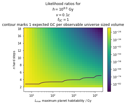
I will address the issue of the compatibility of high and high by looking at the likelihood ratios of pairs of (, ).
I first show a toy model to demonstrate that the deadline effect is weak (but present) and then reproduce the likelihood ratios from my Bayesian model.
My toy model (code here)
I make the following simplifications in this toy likelihood ratio calculation
And the most important assumptions:
Writing & for the PDF & CDF of the Gamma distribution parameters n and h:
Toy model results
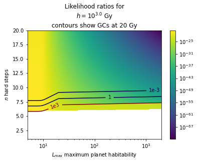 | 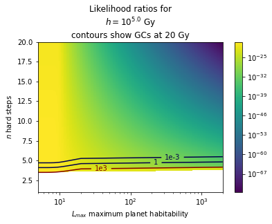 | 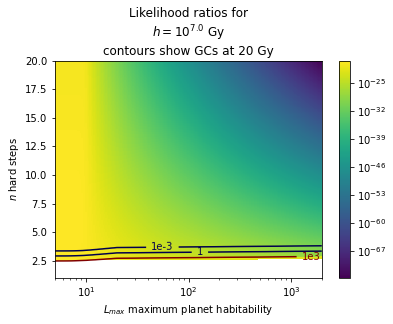 |
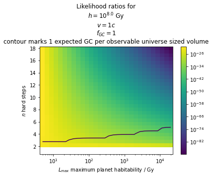
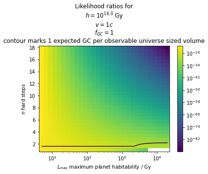
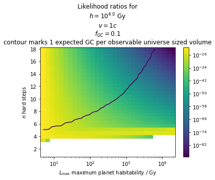
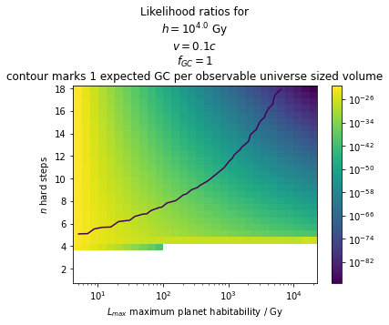
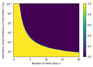
Above: some plot of the likelihood ratios of pairs of . The three plots vary by value of (the geometric mean of the hardness of the steps).
The white areas show where life on Earth is precluded by early arriving GCs.
The contour lines show the (expected) number of GCs at 20 Gy. For more than 1000 GCs at 20 Gy (but not so many to preclude human-like civilizations) there are relatively high likelihood ratios.
For example, has a likelihood ratio 1e-24. In this case there are around 5200 GCs existing by 20 Gy, so the toy deadline effect is triggered. However, this likelihood ratio is much smaller than the case [just shifting along to the left] which has ratio 1e-20. In this latter case, there are 0.4 expected GCs by 20 Gy, so the toy deadline effect is not triggered.
Toy model discussion
This toy deadline effect that can be induced by higher (holding other parameters constant) is not strong enough to compete with humanity becoming increasingly atypical when. Increasing makes Earthlike civilizations less typical by
(1) the count effect, where there are more longer lived planets than shorter lived ones like Earth. In the toy model, this effect accounts for decrease in typicality. This effect is relatively weak.
(2) the power law effect, where the greater habitable duration allows for more attempts at completing the hard steps. When there is a deadline effect at 20 Gy (say) and the universe is habitable from 5 Gy, any planet that is habitable for at least 15 Gy has three times the duration for an IC or GC to appear. For sufficiently hard steps, this effect is roughly decreases life on Earth's typicality by . This effect is weaker when the deadline is set earlier (when there are faster moving GCs).
This second effect can be strong, dependent on when the deadline occurs. At a minimum, if the universe has been habitable since 5 Gy after the Big Bang the deadline effect could occur in the next 1 Gy and there would still be a typicality decrease. The power law effect's decrease on our typicality can be minimised if all planets only became habitable at the same time as Earth.[3]
This toy deadline effect model also shows that it only happens in a very small part of the sample space. This motivates (to me) why the posterior on is so pushed away from high values.
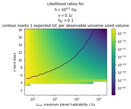
Likelihoods from the full model
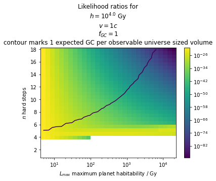
I now show the likelihood ratios for pairs having fixed the other parameters in my model. I set
The deadline effect is visible in all cases. For example, the first graph in 1) with has with likelihood ratio 1.5e-25. Although this is high relative to other likelihood ratios with it is small compared to moving to the left to which has likelihood ratio 3e-22.
1)
The plots differ by value of
 |  |  |  |
2)
 |  |  |  |
3)
 |  |  |  |
4)
 |  |  |  |
For SSA-like updates, this does not in fact matter
Chosen somewhat arbitrarily. I don't think the exact number matters though it should higher for slower expanding GCs.
This also depends on our reference class. I consider the reference class of observers in all ICs, but if we restrict this to observes in ICs that do not observe GCs then we also require high expansion speeds
I got around halfway through. Some random comments, no need to respond:
The possibility of try-once steps allows one to reject the existence of hard try-try steps, but suppose very hard try-once steps.
Typos:
Thanks for your questions and comments! I really appreciate someone reading through in such detail :-)
- What is the highest probability of encountering aliens in the next 1000 years according to reasonable choices once could make in your model?
SIA (with no simulations) gives the nearest and most numerous aliens.
My bullish prior (which has a priori has 80% credence in us not being alone) with SIA and the assumption that grabby aliens are hiding gives a median of ~ chance in a grabby civilization reaching us in the next 1000 years.
I don't condition on us not having any ICs in our past light cone. When conditioning on not being inside a GC, SIA is pretty confident (~80% certain) that we have at least one IC (origin planet) in our past light cone. When conditioning on not seeing any GCs, SIA thinks ~50% that there's at least one IC in our past light cone. Even if there origin planet is in our light cone, they may already be dead.
- Sometimes you just give a prior, e.g., your prior on d, where I don't really know where it comes from. If it wouldn't take too much time, it might be worth it to quickly motivate them (e.g., "I think that any interval between x and y would be reasonable because of such and such, and I fitted a lognormal". It's possible I'm just missing something obvious to those familiar with the literature.
Thanks for the suggestion, this was definitely an oversight. I'll add in some text to motivate each prior.
Lots of the priors aren't super well founded. Fortunately, if you think my bounds on each parameter is reasonable, I get the same conclusions when taking a joint prior that is uniform on and log-uniform in all other parameters.
- Do you think your conclusion (e.g., around likelihood of observing GCs) would change significantly if "non-terrestrial" planets were habitable?
Good question. In a hack-y and unsatisfactory way, my model does allow for this:
If the ratio of non-terrestrial (habitable) planets to terrestrial (habitable) planets is , they replace the product of try-once steps with to account for the extra planets. (My prior on is bounded above by 1, but this could be easily changed). This approach would also suppose that non-terrestrial planets had the same distribution of habitable lifetimes as terrestrial ones.
Having said that, I don't think a better approach would change the results for the SIA and ADT updates. For SSA, the habitability of non-terrestrial planets makes civs like us more atypical (since we are on a terrestrial planet). If this atypicality applies equally in worlds with many GCs and worlds with very few GCs, then I doubt it would change the results. All the anthropic theories would update strongly against the habitability of non-terrestrial planets.
Typos:
Thanks!
My bullish prior (which has a priori has 80% credence in us not being alone) with SIA and the assumption that grabby aliens are hiding gives a median of ~ chance in a grabby civilization reaching us in the next 1000 years.
Don't you mean 1-that?
"
The possibility of try-once steps allows one to reject the existence of hard try-try steps, but suppose very hard try-once steps.
"
Because if (say) only 1/10^30 stars has a planet with just the right initial conditions to allow for the evolution of intelligent life, then that fully explains the Great Filter, and we don't need to posit that any of the try-try steps are hard (of course, they still could be).
Right, thanks
Looks like great work! Do you plan to publish this in a similar venue to previous papers on this topic, such as in an astrophysics journal? I would be very happy to see more EA work published in mainstream academic venues.
Thanks! I've considered it but have not decided whether I will. I'm unsure whether the decision relevant parts (which I see as most important) or weirder stuff (like simulations) would need to be cut.
Hi Tristan,
This is a meta comment (ahaven't had the chance to properly read your paper yet) but this is the kind of document I would have normally expected to encounter as a 50 page LaTeX-generated pdf, and yet I much prefer this format! A pet peeve of mine is that so much quantitative research is latex/pdf based and I deeply dislike essentially all latex software.
May I ask how you went about writing and formatting this? What format/program did you use to draft it? (my first guess is some kind of markdown) Was it easy to format for EA forum? Did you use any neat tricks for embedding code output (e.g. with rmarkdown)?
May I ask how you went about writing and formatting this? What format/program did you use to draft it? (my first guess is some kind of markdown) Was it easy to format for EA forum? Did you use any neat tricks for embedding code output (e.g. with rmarkdown)?
Not the OP, but I usually start in markdown, convert it to html using pandoc (with the -r gfm). Then I copy the html to Google docs, share it with people, rework it after their comments, post it to the EA forum, and then download an html from the forum's graphql API which I convert to markdown for my own archives.
This definitely sounds like a better approach than mine, thanks for sharing! This will be useful for me for any future projects
Thanks, glad to hear it!
I wrote it in Google Docs, primarily for the ease of getting comments. I then copied it into the EA Forum editor and spent a few hours fixing the formatting - all the maths had to be rewritten, all footnote added back in, tables fixed, image captions added - which was a bit of a hassle.
I sadly don't have any neat tricks. I tried this Google Docs tool to convert to Markdown but it didn't work well.
The EA Forum editor now have the ability to share drafts and allow comments and collaborative editing, which I think I'll try for my next project. I'm also hoping Google Docs will add a better maths editor.
It seems plausible a significant fraction of ICs will choose to become GCs. Since matter and energy are likely to be instrumentally useful to most ICs, expanding to control as much volume as they can (thus becoming a GC) is likely to be desirable to many ICs with diverse aims.
Also, if an IC is a mixture of grabby and non-grabby elements, it will become a GC essentially immediately.
+1
I think Hanson et al. mention something like this too
If you had to remake this 3D sim of the expansion of grabby aliens based on your beliefs, what would look different, exactly? (Sorry, I know you already answer this indirectly throughout the post, at least partially.)
dude 1 year later and holy shit you did your research, so glad we have people like you able to look at this stuff like this.

Crossposted to LessWrong
This report is the most comprehensive model to date of aliens and the Fermi paradox. In particular, it builds on Hanson et al. (2021) and Olson (2015) and focuses on the expansion of ‘grabby’ civilizations: civilizations that expand at relativistic speeds and make visible changes to the volume they control.
This report considers multiple anthropic theories: the self-indication assumption (SIA), as applied previously by Olson & Ord (2022), the self-sampling assumption (SSA), implicitly used by Hanson et al. (2021) and a decision theoretic approach, as applied previously by Finnveden (2019).
In Chapter 1, I model the appearance of intelligent civilizations (ICs) like our own. In Chapter 2, I consider how grabby civilizations (GCs) modify the number and timing of intelligent civilizations that appear.
In Chapter 3 I run Bayesian updates for each of the above anthropic theories. I update on the evidence that we are in an advanced civilization, have arrived roughly 4.5Gy into the planet’s roughly 5.5 Gy habitable duration, and do not observe any GCs.
In Chapter 4 I discuss potential implications of the results, particularly for altruists hoping to improve the far future.
Starting from a prior similar to Sandberg et al.’s (2018) literature-synthesis prior, I conclude the following:
Using SIA or applying a non-causal decision theoretic approach (such as anthropic decision theory) with total utilitarianism, one should be almost certain that there will be many GCs in our future light cone.
Using SSA[1], or applying a non-causal decision theoretic approach with average utilitarianism, one should be confident (~85%) that GCs are not in our future light cone, thus rejecting the result of Hanson et al. (2021). However, this update is highly dependent on one’s beliefs in the habitability of planets around stars that live longer than the Sun: if one is certain that such planets can support advanced life, then one should conclude that GCs are most likely in our future light cone. Further, I explore how an average utilitarian may wager there are GCs in their future light cone if they expect significant trade with other GCs to be possible.
These results also follow when taking (log)uniform priors over all the model parameters.
All figures and results are reproducible here.
To set the scene, I start with two vignettes of the future. This section can be skipped, and features terms I first explain in Chapters 1 and 2.
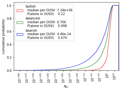
In a Monte Carlo simulation of draws, the following world described gives the highest likelihood for both SIA and SSA (with reference class of observers in intelligent civilizations). That is, civilizations like ours are both relatively common and typical amongst all advanced-but-not-yet-expansive civilizations in this world.
In this world, life is relatively hard. There are five hard try-try steps of mean completion time 75 Gy, as well as 1.5 Gy of easy ‘delay’ steps. Planets around red dwarfs are not habitable, and the universe became habitable relatively late -- intelligent civilizations can only emerge from around 8 Gy after the Big Bang. Around 0.3% of terrestrial planets around G-stars like our own are potentially habitable making Earth not particularly rare.
Around 2.5% intelligent civilizations like our own become grabby civilizations (GCs). This is the SIA Doomsday argument in action.
Around 7,000 GCs appear per observable universe sized volume (OUSV). GCs already control around 22% of the observable universe, and as they travel at , their light has reached around 35% of the observable universe. Nearly all GCs appear between 10Gy and 18 Gy after the Big Bang.
If humanity becomes a GC, it will be slightly smaller than a typical GC - around 62% of GCs will be bigger. A GC emerging from Earth would in expectation control around 0.1% of the future light cone and almost certainly contain the entire Laniakea Supercluster, itself containing at least 100,000 galaxies.

The median time by which GCs will be visible to observers on Earth is around 1.5 Gy from now. It is practically certain humanity will not see any GCs any time soon: there is roughly 0.000005% probability (one in twenty million) that light from GCs reaches us in the next one hundred years[2]. GCs will certainly be visible from Earth in around 4 Gy.
As we will see, SIA is highly confident in a future is similar to this one. SSA (with the reference class of observers in intelligent civilizations), on the other hand, puts greater posterior credence in human civilization being alone, even though worlds like these have high likelihood.
This world is one that a total utilitarian using anthropic decision theory would wager being in, if they thought their decisions can influence the value of the future in proportion to the resources that an Earth originating GC controls.
In this world, there are eight hard steps, with mean hardness 23 Gy and delay steps totalling 1.8 Gy. Planets capable of supporting advanced life are not too rare: around 0.004% of terrestrial planets are potentially habitable. Again, planets around longer-lived stars are not habitable.
Around 90% of ICs become GCs, and there are roughly 150 GCs that appear per observable universe sized volume. GCs expand at 0.85c, and a GC emerging from Earth would reach 31% of our future light cone, around 49% of its maximum volume, and would be bigger than ~80% of all GCs. Since there are so few GCs, the median time by which a GC is visible on Earth is not for another 20 Gy.

I use the term intelligent civilizations (ICs) to describe civilizations at least as technologically advanced as our own.
In this chapter, I derive a distribution of the arrival times of ICs, . This distribution is dependent on factors such as the difficulty of the evolution of life and the number of planets capable of supporting intelligent life. This distribution does not factor in the expansion of other ICs, that may prevent (‘preclude’) later ICs from existing. That is the focus of Chapter 2.
The distribution gives the number of other ICs that arrive at the same time as human civilization, as well as the typicality of the arrival time of human civilization, assuming no ICs preclude any other.
I write for the time since the Big Bang, which is estimated 13.787 Gy (Ade 2016) [Gy = gigayear = 1 billion years].
Current observations suggest the universe is most likely flat (the sum of angles in a triangle are always 180°), or close to flat, and so the universe is either large or infinite. Further, the universe appears to be on average isotropic (there are no special directions in the universe) and homogeneous (there are no special places in the universe) (Saadeh et al. 2016, Maartens 2011).
The large or infinite size implies that there are volumes of the universe causally disconnected from our own. The collection of ‘parallel’ universes has been called the “Level I multiverse”. Assuming the universe is flat, Tegmark (2007) conservatively estimates that there is a Hubble volume identical to ours away, and an identical copy of you away.
I consider a large finite volume (LFV) of the level I multiverse, and partition this LFV into observable universe size (spherical) volumes (OUSVs)[3] . My model uses quantities as averages per OUSV. For example, will be the rate of ICs arriving per OUSV on average at time .
The (currently) observable universe necessarily defines the limit of what we can currently know, but not what we can eventually know. The eventually observable universe has a volume around 2.5 times that of the volume of the currently observable universe (Ord 2021).
The most action relevant volume for statistics about the number of alien civilizations is the affectable universe, the region of the universe that we can causally affect. This is around 4.5% of the volume of the observable universe. I will use the term affectable universe size volumes (AUSVs).
For an excellent discussion on this topic, I recommend Ord (2021).
I consider the path to an IC as made up of a number of steps:
I recommend Eth (2021) for an excellent introduction to try-try steps.
Abiogenesis is the process by which life has arisen from non-living matter. This process may require some extremely rare configuration of molecules coming together, such that one can model the process as having some rate 1/a of success per unit time on an Earth-sized planet.
The completion time of such a try-try step is exponentially distributed with PDF . Fixing some time , such as Earth’s habitable duration, the step is said to be hard if . When the step is hard, for , is constant since .
Abiogenesis is one of many try-try steps that have led to human civilization. If there are try-try steps with expected times of completion, the completion time of the steps has hypoexponential distribution with parameter . For modelling purposes, I split these try-try steps into delay steps and hard steps.
I define the delay steps to be the maximal set of individual steps from the steps such that , the approximate duration life has taken on Earth so far. I then approximate the completion time of the delay try-try steps with the exponential distribution with parameter . If they exist, I also include any fuse steps[4] in the sum of .
I write for the expected completion times of the remaining steps. These steps are not necessarily hard with respect to Earth's habitable duration. I model each to have log-uniform uncertainty between 1 Gy and Gy. With this prior, most are much greater than 5 Gy and so hard. I approximate the completion time of all of these steps with the Gamma distribution parameters and , the geometric mean hardness of the try-try steps.[5] The Gamma distribution can further be described as a ‘power law’ as I discuss in the appendix.
I write for the PDF of the completion time of all the delay steps and hard try-try steps. Strictly, it is given as the convolution of the gamma distribution parameters , and exponential distribution parameter . When , where is the PDF of the Gamma distribution. That is, the delay steps can be approximated as completing in their expected time when they are sufficiently short in expectation.
Priors on
After introducing each model parameter, I introduce my priors. Crucially, all the results in Chapter 3 roughly follow when taking (log)uniform priors over all parameters and so my particular prior choices are not too important.
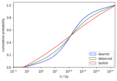
I consider three priors on , the number of hard try-try steps. The first, which I call balanced, is chosen to give an implied prior number of ICs similar to existing literature estimates (discussed later in this chapter). My bullish prior puts greater probability mass on fewer hard steps and so implies a greater number of ICs. My bearish prior puts greater probability mass in many hard steps and so predicts fewer ICs.

My priors on are uninformed by the timing of life on Earth, but weakly informed by discussion of the difficulty of particular steps that have led to human civilization. For example, Sandberg et al. (2018) (supplement I) consider the difficulty of abiogenesis. In Chapter 3 I update on the time that all the steps are completed (i.e., now). I do not update on the timing of the completion of any potential intermediate hard steps, such as the timing of abiogenesis. Further, I do not update on the habitable time remaining, which is implicitly an anthropic update. I discuss this in the appendix.
Prior on
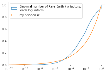
Given these priors on , I derive my prior on by the geometric mean of draws from the above-mentioned . I chose this prior to later give estimates of life in line with existing estimates. A longer tailed distribution is arguably more applicable.

Prior on
My prior on the sum of the delay and fuse steps has . By definition and d smaller than 0.1 Gy makes little difference. My prior distribution gives median . The delay parameter can also include the delay time between a planet's formation and the first time it is habitable. On Earth, this duration could have been up to 0.6 Gy (Pearce et al. (2018)).
I also model “try-once” steps, those that either pass or fail with some probability. The Rare Earth hypothesis is an example of a try-once step. The possibility of try-once steps allows one to reject the existence of hard try-try steps, but suppose very hard try-once steps.
I write for the probability of passing through all try-once steps. That is, if there are try-once steps then
The parameters above give can give distribution of appearance times of an IC on a given planet. In this section, I consider the maximum duration planets can be habitable for, the number of potentially habitable planets, and the formation of stars around which habitable planets can appear.
I write [6] for the maximum duration any planet is habitable for.[7] The Earth has been habitable for between 4.5 Gy and 3.9 Gy (Pearce 2018) and is expected to be habitable for another~1 Gy, so as a lower bound ⪆ 5 Gy. Our Sun, a G-type main-sequence star, formed around 4.6 Gy ago and is expected to live for another ~5 Gy.
Lower mass stars, such as K-type stars (orange dwarfs) have lifetimes between 15 -30 Gy , and M-type stars (red dwarfs) have lifetimes up to 20,000 Gy. These lifetimes give an upper bound on the habitable duration of planets in that star’s system, so I consider up to around 20,000 Gy.
The habitability of these longer-lived stars is uncertain. Since red dwarf stars are dimmer (which results in their longer lives), habitable planets around red dwarf stars must be closer to the star in order to have liquid water, which may be necessary for life. However, planets closer to their star are more likely to be tidally locked. Gale (2017) notes that “This was thought to cause an erratic climate and expose life forms to flares of ionizing electro-magnetic radiation and charged particles.” but concludes that in spite of the challenges, “Oxygenic Photosynthesis and perhaps complex life on planets orbiting Red Dwarf stars may be possible”.

This approach to modelling does not allow for planets around red dwarf stars that are habitable for periods equal to the habitable period of Earth. For example, life may only be able to appear in a crucial window in a planet’s lifespan.
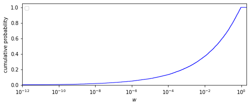
Given a value of , I now consider the number of habitable planets. To derive an estimate of the number of potentially habitable planets, I only consider the number of terrestrial planets: planets composed of silicate rocks and metals with a solid surface. Recall that the parameter w can indirectly control the number of these actually habitable.
Zackrisson et al. (2016) estimate terrestrial planets around FGK stars and around M stars in the observable universe. Interpolating, I set the total number of terrestrial planets around stars that last up to per OUSV to be
Hanson et al. (2021) approximate the cumulative distribution of planet lifetimes with for and for . The fraction of planets formed at time habitable at time t is then given by .
These forms of and satisfy the property that for any, the expression - the number of planets per OUSV habitable for between and Gy - is independent of . In particular, the number of planets habitable for the same duration as Earth is independent of .
This is implicitly used later in the update: one does not need to explicitly condition on the observation that we are on a planet with habitable for ~5 Gy since the number of planets habitable for ~5 Gy is independent of the model parameters.
I use the term “habitable stars” to mean stars with solar systems capable of supporting life.
I follow Hanson et al. (2021) in approximating the habitable star formation rate with the functional form with power and decay where .

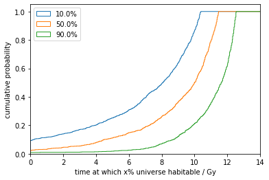
There is debate over the time the universe was first habitable.
Loeb (2016) argues for the universe being habitable as early as 10 My. There is discussion around how much gamma-ray bursts (GBRs) in the early universe prevent the emergence of advanced life. Piran (2014) conclude that the universe was inhospitable to intelligent life > 5 Gy ago. Sloan et al. (2017) are more optimistic and conclude that life could continue below the ground or under an ocean.
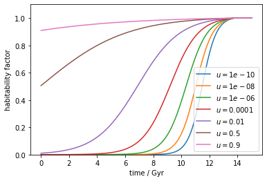
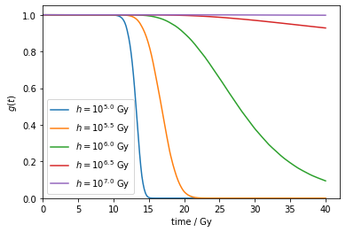
I introduce an early universe habitability parameter and function which gives the fraction of habitable planets capable of hosting advanced life at time relative to the fraction at . I take to be a sigmoid function with and (hence ). My prior on is log-uniform on (, 0.99)
A more sophisticated approach would consider the interaction between and the hard try-try steps, as suggested by Hanson et al. (2021).
The number of planets terrestrial planets per OUSV habitable at time is
Since for , the lower bound of the integral can be changed to .
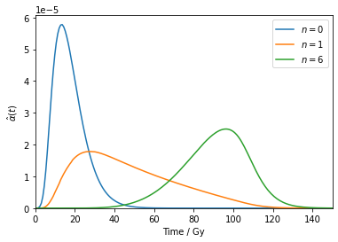
Putting the previous sections together, the appearance rate of ICs per OUSV, , is given by
To recap:
I now discuss two potential puzzles related to : Did humanity arrive at an unusually early time? And, where are all the aliens?
Depending on one’s choice of anthropic theory, one may update towards hypotheses where human civilization is more typical among the reference class of all ICs.
Here, I look at human civilization’s typicality using two pieces of data: human civilization’s arrival at and the fact that we have appeared on a planet habitable for ~5 Gy.
An atypical arrival time?
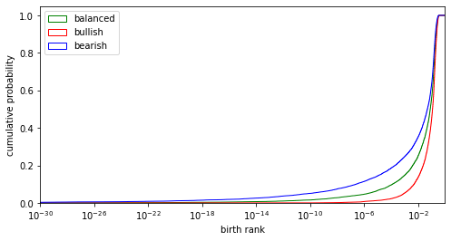
I write for the arrival time distribution normalised to be a probability density function. This tells us how typical human civilization’s arrival time is. That is, is the probability density of a randomly chosen (eventually) existing IC to have arrived at .
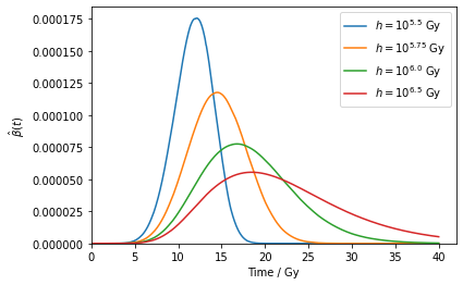
 |  |
Plots of for varying , all with , , and .. The left-hand plots have and right hand plots have . When planets are habitable for a longer duration, a greater fraction of life appears later. Further, when is greater, fewer ICs appear overall since life is harder, but a greater fraction of ICs appear later in their planets’ habitable windows – this is the power law of the hard steps. | |

An atypical solar system?
There are many more terrestrial planets around red dwarf stars than stars like our own. If these systems are habitable, then human civilization is additionally atypical (with respect to all ICs) in its appearance around a star like our sun. Further, life has a longer time to evolve around a longer lived star, so human civilization would be even more atypical. Haqq-Misra et al. (2018) discuss this, but do not consider that the presence of hard try-try steps leads to a greater fraction of ICs appearing on longer-lived planets.
Resolving the paradox
Suppose a priori one believes and and uses an anthropic theory that updates towards hypotheses where human civilization is more typical among all ICs. Given these assumptions, one expects the vast majority of ICs to appear much further into the future and on planets around red dwarf stars. However, human civilization arrived relatively shortly after the universe first became habitable, on a planet that is habitable for only a relatively short duration and is thus very atypical (according to our arrival time function that does not factor in the preclusion of ICs by other ICs.
There are multiple approaches to resolving this apparent paradox.
First, one can reject their prior belief in high and , and update towards small and which lead us to believing we are in a more typical IC.
Second, one could change the reference class among which human civilization’s typicality is being considered. This, in effect, is changing the question being asked.[8]
Third and finally, one can prefer theories that set a deadline on the appearance of ICs like us. If the universe suddenly ended in 5 Gy time, no more ICs could appear and regardless of n and human civilization’s arrival time would be typical.
Hanson et al. (2021) resolve the paradox with such a deadline, the expansion of so-called grabby civilizations, which is the focus of Chapter 2. Alternative deadlines have been suggested, such as through false vacuum decay, which I briefly discuss in the appendix.
Some anthropic theories update towards hypotheses where there are a greater number of civilizations that make the same observations we do (containing observers like us).
The rate of XICs
I write for the rate of ICs per OUSV with feature X, where X denotes “ICs arriving at tnow on a planet that has been habitable for as long as Earth has, and will be habitable for the same duration as Earth will be".
The Earth has been habitable for between 4.5 Gy and 3.9 Gy (Pearce et al. 2018). I suppose that Earth has been habitable for 4.5 Gy, since if habitable for just 3.9 Gy, the 600 My difference can be (lazily) modelled as a fuse or delay step. Assuming for the time being that no IC precludes any other, this gives
Note that
Below, I vary and to see the effect on . The effect of on is linear, so uninteresting.

The term does not include the further feature of not observing any alien life. In the next chapter, I introduce the number of ICs with feature X that also do not observe any alien life.
Where are all the aliens?
I write for the rate of ICs that appear per OUSV, supposing no IC precludes any other, which is given by .
My priors on , , , , and give the rate of ICs that appear per OUSV, supposing no IC precludes any other.
I chose the balanced prior on and prior on hard step hardness to give an implied distribution on comparable to the prior derived by Sandberg et al. (2018), which models the scientific uncertainties on the parameters of the Drake Equation. Sandberg et al.’s prior on the number of currently contactable ICs has a median of 0.3 and 38% credence in fewer than one IC currently existing in the observable universe. My balanced prior gives ~50% on the rate of less than one IC per OUSV and median of ~1 IC to appear per OUSV, and so is more conservative.
The Fermi observation is the fact that we have not observed any alien life. For those with a high prior on the existence of alien life, such as my bullish prior, the Fermi paradox is the conflict between this high prior and the Fermi observation.
It may be hard for humanity to observe a typical IC, especially if they do not last long or emit enough electromagnetic radiation to be identified at large distances. If some fraction of ICs persist for a long time, expand at relativistic speeds, and make visible changes to their volumes, one can more easily update on the Fermi observation. Such ICs are called grabby civilizations (GCs).
The existence of sufficiently many GCs can ‘solve’ the earliness paradox by setting a deadline by which ICs must arrive, thus making ICs like us more typical in human civilization’s arrival time.
In this chapter, I derive an expression for , the rate of ICs per OUSV that have arrived at the same time as human civilization on a planet habitable for the same duration and do not observe any GCs.
Humanity has not observed any intelligent life. In particular, we have not observed any GCs.
Whether GCs are not in our past light cone or we have not yet seen them yet is uncertain. GCs may deliberately hide or be hard to observe with humanity’s current technology.
It seems clearer that humanity is not inside a GC volume, and at minimum we can condition on this observation.[9]
In Chapter 3 I compute two distinct updates: one conditioning on the observation that there are no GCs in our past light cone, and one conditioning on the weaker observation that we are not inside a GC volume. If GCs prevent any ICs from existing in their volume, this latter observation is equivalent to the statement that “we exist in an IC”.
The second observation leaves ‘less room’ for GCs, since we are conditioning on a larger volume not containing any GCs.
I lean towards there being no GCs in our past light cone. By considering the waste heat that would be produced by Type III Kardashev civilizations (a civilization using all the starlight of its home galaxy), the G-survey found no type III Kardashev civilizations using more than 85% of the starlight in 105 galaxies surveyed (Griffith et al. 2015). There is further discussion on the ability to observe distant expansive civilizations in this LessWrong thread.
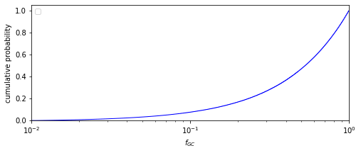
I write for the average fraction of ICs that become GCs.[10] I assume that this happens in an astronomically short duration and as such can approximate the distribution of arrival time of GCs as equal to the distribution of arrival times of ICs. That is, the arrival time distribution of GCs is given by .
It seems plausible a significant fraction of ICs will choose to become GCs. Since matter and energy are likely to be instrumentally useful to most ICs, expanding to control as much volume as they can (thus becoming a GC) is likely to be desirable to many ICs with diverse aims. Omohundro (2008) discusses instrumental goals of AI systems, which I expect will be similar to the goals of GCs (run by AI systems or otherwise).
Some ICs may go extinct before being able to become a GC. The extinction of an IC does not entail that no GC emerges. For example, an unaligned artificial intelligence may destroy its origin IC but become a GC itself. (Russell 2021). ICs that trigger a (false) vacuum decay that expands at relativistic speeds can also be modelled as GCs.
I do not update on the fact we have not observed any ICs. The smaller , the greater the importance of the evidence that we have not seen any ICs.
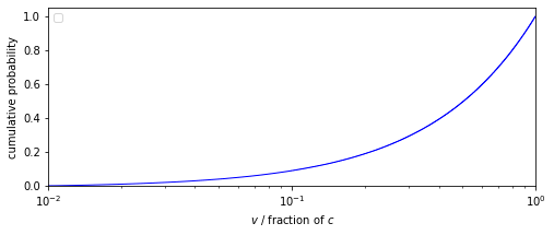
I model GCs as all expanding spherically at some constant comoving speed .
To calculate the volume of an expanding GC, one must factor in the expansion of the universe.
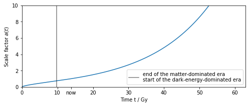
Solving the Friedmann equation gives the cosmic scale factor , a function that describes the expansion of the universe over time.
With initial condition and , , and given by Ade et al. (2016). The Friedmann equation assumes the universe is homogeneous and isotropic, as discussed in Chapter 1.
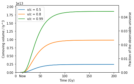
Throughout, I use comoving distances which give a distance that does not change over time due to the expansion of space. The comoving distance a probe travelling at speed that left at time reaches by time is .The comoving volume of a GC at time that has been growing at speed since time is
I take in units of fraction of the volume of an OUSV, approximately .
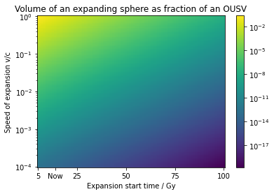
Following Olson (2015) I write for the average fraction of OUSVs unsaturated by GCs at time and take functional form
Recall that the product is the rate of GCs appearing per OUSV at time . Since is a function of the parameters ,,, , and , the function is too.
This functional form for assumes that when GCs bump into other GCs, they do not speed up their expansion in other directions.
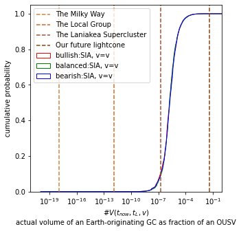
The actual volume of a GC
I write for the expected actual volume of a GC at time that began expanding at time at speed . Trivially, since GCs that prevent expansion can only decrease the actual volume. If GCs are sufficiently rare, then . I derive an approximation for in the appendix.
Later, I use the actual volume of a GC as a proxy for the total resources it contains. On a sufficiently large scale, mass (consisting of intergalactic gas, stars, and interstellar clouds) is homogeneously distributed within the universe. This proxy most likely underweights the resources of later arriving GCs due to the gravitational binding of galaxies and galaxy-clusters.

The distribution of IC arrival times,, can be adjusted to account for the expansion of GCs, which preclude ICs from arriving. I define that gives the rate of ICs appearing per OUSV, and write for the number of ICs that actually appear per OUSV.


I define to be the actual number of ICs with feature X to appear, accounting for the expansion of GCs. I consider two variants of this term.
I write for the rate of ICs with feature X per OUSV that do not observe GCs. Since information about GCs travels at the speed of light, gives the fraction of OUSVs that is unsaturated by light from GCs at time . Then, gives the number of XICs per OUSV with no GCs in their past light cone.
Similarly, I write [11]for the rate of ICs with feature X per OUSV that are not inside a GC volume, where v is the expansion speed of GCs. In this case, .
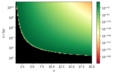 |  |
Left and right: heatmaps of for varying hard steps and geometric mean hardness . Both heatmaps show the same data, but the colour scale goes with the logarithm on the plot on the left, and linearly on the right. Both take ,, , , and . The black area in the left heatmap contains pairs of such that no XICs actually appear, due to the all OUSVs being saturated by light from GCs by . The green area on the right heatmap is the 'sweet spot' where the most number of XICs appear. This happens to be just above the border between the black and green area in on the left heatmap. In this ‘sweet-spot’, there are many ICs (including XICs) but not too many such that XICs are (all) precluded. My bearish, balanced and bullish priors have 16%, 26% and 44% probability mass in cases where the universe is fully saturated with light from GCs by (and so ) respectively. | |
The Fermi observation limits the number of early arriving GCs: when there are too many GCs the existence of observers like us is rare or impossible.
For anthropic theories that prefer more observers like us, there is a push in the other direction. If life is easier, there will be more XICs.
For anthropic theories that prefer observers like us to be more typical, there is potentially a push towards the existence of GCs that set a cosmic deadline and lead to human civilization not being unusually early.
In the next chapter, I derive likelihood ratios for different anthropic theories and produce results.
I’ve presented all the machinery necessary for the updates, other than the anthropic reasoning. I hope this chapter is readable without knowledge of the previous two.
I now apply three approaches to dealing with anthropics:
I have three joint priors over the following eight parameters.
I update on either the observation I label or observation I label . Both and include observing that we are in an IC that
additionally contains the observation that we do not see any GCs. Alternatively, additionally contains the observation that we are not inside a GC (equivalently, that we exist, if we expect GCs to prevent ICs like us from appearing).
I walk through each anthropic theory in turn, derive a likelihood ratio, and produce results. In Chapter 4 I discuss potential implications of these results.
By Bayes rule
I have already given my priors and so it remains to calculate the likelihood P(X|n, ..., v). I derive likelihoods in the discrete case, and index my priors by worlds .
I use the following definition of the self-indication assumption (SIA), slightly modified from Bostrom (2002)
All other things equal, one should reason as if they are randomly selected from the set of all [12]possible observer moments (OMs) [a brief time-segment of an observer].[13]
Applying the definition of SIA,
That is, SIA updates towards worlds where there are more OMs like us. Since the denominator is independent of , we only need to calculate the numerator, .
By my choice of definitions, is proportional to , the number of ICs with feature X that actually appear per OUSV. The constant of proportionality is given by the number of OMs per IC, which I suppose is independent of model parameters, as well as the number of OUSVs in the earlier specified large finite volume. Again, these constants is unnecessary due to the normalisation.
The three summary statistics implied by the posterior are below. As mentioned before, the updates are reproducible here.
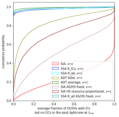
| Updating with observation Xc | Updating with observation Xv |
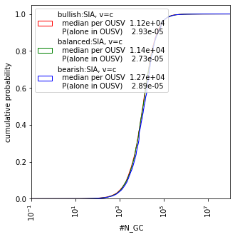 |  |
 |  |
 |  |
SIA updates overwhelmingly towards the existence of GCs in our light cone from all three of my priors. If a GC does not emerge from Earth, most of the volume will be expanded into by other GCs.
I discuss some marginal posteriors here, and reproduce all the marginal posteriors in the appendix.
SIA updates towards smaller as the existence of more GCs can only decrease the number of observers like us. This is the “SIA Doomsday” described by Grace (2010). This result is the same as found by Olson & Ord (2021) whereby the prior on goes from prior to posterior .
The SIA update is overwhelmingly towards smaller . Increasing only increases the number of GCs that could preclude XICs.


I use the following definition of the self-sampling assumption (SSA), again slightly modified from Bostrom (2002)
All other things equal, one should reason as if they are randomly selected from the set of all actually existent observer moments (OMs) in their reference class.[14]
A reference class is a choice of some subset of all OMs. Applying the definition of SSA with reference class ,
That is, SSA updates towards worlds where observer moments like our own are more common in the reference class.
I first consider two reference classes, and . The reference class contains only OMs contained in ICs, and no OMs in GCs. This is the reference class implicitly used by Hanson et al. (2021). The reference class also includes observers in GCs. I later consider the minimal reference class, containing only observers who have identical experiences, paired with non-causal decision theories.
This is the reference class implicitly used by Hanson et al. (2021). I reach different conclusions from Hanson et al. (2021), and discuss a possible error in their paper in the appendix.
The total number of OMs in is proportional to the number of ICs, . As in the SIA case, the number of XOMs is proportional to , so the likelihood ratio is .
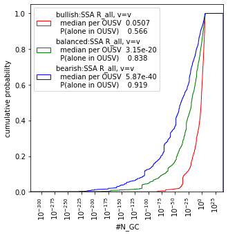
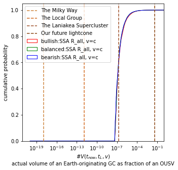
| Updating with observation Xc | Updating with observation Xv |
 |  |
 |  |
 |  |
SSA has updated away from the existence of GCs in our future light cone.
In the appendix, I discuss how this update is highly dependent on the lower bound on the prior for . Again, smaller is unsurprisingly preferred.

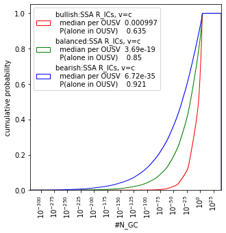
This reference class contains all OMs that actually exist in our large finite volume, and so includes OMs that GCs create. It is sometimes called the “maximal” reference class[15].
I model GCs as using some fraction of their total volume to create OMs. I suppose that this fraction and the efficiency of OM creation are independent of the model parameters. These constants do not need to be calculated, since they cancel when normalising.
The total volume controlled by all GCs is proportional to , the average fraction of OUSVs saturated by GCs at some time when all expansion has finished[16].
I assume that a single GC creates many more OMs than are contained in a single ICs. Since my prior on has and I expect GCs to produce many OMs, I see this as a safe assumption. This assumption implies the total number of OMs as proportional to . The SSA likelihood ratio is .
I do not see this update as not particularly informative, since I expect GCs to create simulated XOMs., which I explore later in this chapter.
| Updating with observation Xc | Updating with observation Xv |
 |  |
 |  |
 |  |
Notably, SSA updates towards as small as possible, since increasing the speed of expansion increases the number of observers created that are not like us — the denominator in the likelihood ratio.
As with the SSA update, this result is sensitive to the prior on , which I discuss in the appendix.
In this section, I apply non-causal decision theoretic approaches to reasoning about the existence of GCs. This chapter does not deal with probabilities, but with ‘wagers’. That is, how much one should behave as if they are in a particular world.
The results I produce are applicable to multiple non-causal decision theoretic approaches.
The results are applicable for someone using SSA with the minimal reference class () paired with a non-causal decision theory, such as evidential decision theory (EDT). SSA contains only observers identical to you, and so updating using SSA Rmin simply removes any world where there are no observers with the same observations as you, and then normalises.
The results are also applicable for someone (fully) sticking with their priors (being ‘updateless’) and using a decision theory such as anthropic decision theory (ADT). ADT, created by Armstrong (2011), converts questions about anthropic probability to decision problems, and Armstrong notes that “ADT is nothing but the Anthropic version of the far more general ‘Updateless Decision Theory’ and ‘Functional Decision Theory’”.
I suppose that all decision relevant ‘exact copies’ of me (i.e. instances of my current observations) are in one of the following situations
Of course, copies may be in non-decision relevant situations, such as short-lived Boltzmann brains.
For each of the above three situations, I calculate the expected number of copies of me per OUSV. For example, in case (1), the number of copies is proportional to and in (2) [18]. I do not calculate the constant of proportionality (which would be very small) - this constant is redundant when considering the relative decision worthiness of different worlds.
My decisions may correlate with agents that are not identical copies of me (at a minimum, near identical copies) which I do not consider in this calculation. If in all situations the relative increase in decision-worthiness from correlated agents is equal, the overall relative decision worthiness is unchanged.
To motivate the need to consider these three cases, I claim that our decisions are likely contingent on the ratio of our copies in each category and the ratio of the expected utility of our possible decisions in each scenario. For example, if we were certain that none of our copies were in ICs that became GCs, or all of our copies were in short-lived simulations, we may prioritise improving the lives of current generations of moral patients.
The GC wager
I choose to model all the expected utility of our decisions as coming from copies in case (1). That is, to make decisions premised on the wager that we are in an IC that becomes a GC and not in an IC that doesn’t become a GC, nor in a short-lived simulation.
Tomasik (2016) discusses the comparison of decision-worthiness between (1) and (2) to (3). My assumption that (1) dominates (2) is driven by my prior distribution on fGC (which is bounded below by 0.01) and the expected resources of a single GC dominating the resources of a single IC.
Counterarguments to this assumption may appeal to the uncertainty about the ability to affect the long-run future. For example, if a GC emerged from Earth in the future but all the consequences of one’s actions ‘wash out’ before that point, then (1) and (2) would be equally decision-worthy.
I expect that forms of lock-in, such as the values of an artificial general intelligence, provide a route for altruists to influence the future. I suppose that a total utilitarian’s decisions matter more in cases where the Earth emerging GC is larger. In fact, I suppose a total utilitarian’s decisions matter in linear proportion to the eventual volume of such a GC.
An average utilitarian’s decisions then matter in proportion to the ratio of the eventual volume of an Earth emerging GC to the volume controlled by all GCs, supposing that GCs create moral patients in proportion to their resources.
Calculating decision-worthiness
To give my decision worthiness of each world, I multiply the following terms:
This gives the degree to which I should wager my decisions on being in a particular world.
Total utilitarianism
The number of copies of me in ICs that become GCs is proportional to. The expected actual volume of such GCs is . Using the assumption that our influence is linear in resources, the decision worthiness of each world is
I use the label “ADT total” for this case.
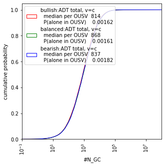
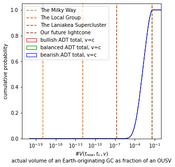
| Updating with observation | Updating with observation |
 |  |
 |  |
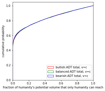 |  |
Total utilitarians using a non-causal decision theory should behave as if they are almost certain of the existence of GCs in their future light cone. However, the number of GCs is fairly low - around 40 per AUSV.
Average utilitarianism
As before, the number of copies of me in ICs that become GCs is proportional to and again the expected actual volume of such a GC is given by The resources of all GCs is proportional to . Supposing that GCs create moral patients in proportion to their resources, the decision worthiness of each world is
I use the label “ADT average” for this case.
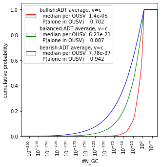
| Updating with observation | Updating with observation |
 | 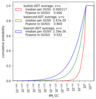 |
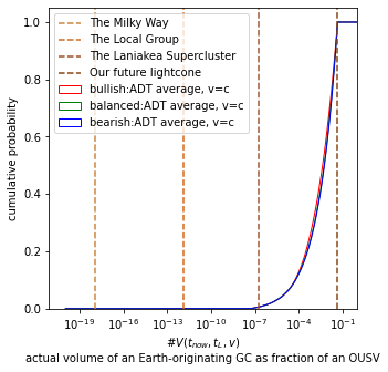 |  |
 | 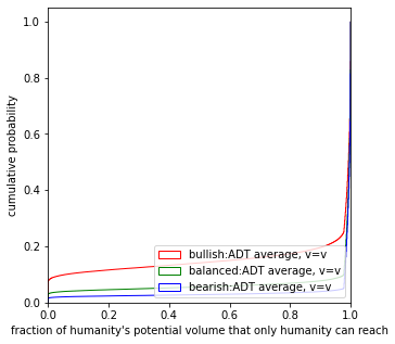 |
An average utilitarian should behave as if there are most likely no GCs in the future light cone. As with the SSA updates, this update is sensitive to the prior on and is explored in an appendix.
I now model two types of interactions between GCs: trade and conflict.
The model of conflict that I consider decreases the decision worthiness of cases where there are GCs in our future light cone. I show that a total utilitarian should wager as if there are no GCs in their future light cone if they think the probability of conflict is sufficiently high.
The model of trade I consider increases the decision worthiness of cases where there are GCs in our future light cone. I show that an average utilitarian should wager that there are GCs in their future light cone if they think there are sufficiently large gains from trade with other GCs.
The purpose of these toy examples is to illustrate that a total or average utilitarian’s true wager with respect to GCs may be more nuanced than presented earlier.
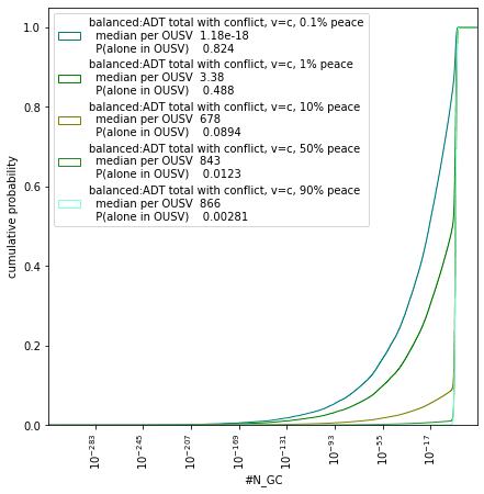
Total utilitarianism and conflict
Suppose we are in the contrived case where:
When conflict occurs, an Earth originating GC has probability [20]of getting its maximal volume, . Supposing a total utilitarian’s decisions can influence both cases equally, the expected decision-worthiness per copy in an IC that becomes a GC is
As before, multiplying by the number of copies of me in ICs that become GCs, , gives the decision worthiness.
Intuitively, since the conflict in expectation is a net loss of resources for all GCs, this leads one to wager one’s decisions against the existence of GCs in the future.
Average utilitarianism and trade
I apply a very basic model of gains from trade between GCs with average utilitarianism. I suppose that one can only trade with other GCs within the affectable universe.[21][22]
Intuitively the decision worthiness goes up in a world with trade as there is more at stake: our GC can both influence its own resources and the resources of other GCs. This model of trade would also increase the degree to which a total utilitarian would wager there are GCs in their future light cone.
I suppose an average utilitarian GC completes a trade by spending of their resources (which they could otherwise use to increase the welfare of moral patients by a single unit) for the return of welfare of moral patients to be increased by one unit. For the GC benefits by making the trade, and so should always make such a trade rather than using the resources to create utility themselves. I write for the probability density of a randomly chosen trade providing return, and suppose that the ‘volume’ of available trades is proportional to the volume saturated by GCs, which itself is proportional to .
I take for some . For smaller , a greater proportion of all available trades are beneficial, and a greater number are very beneficial. For example, for k=1 the fraction of the volume controlled by GCs that the average utilitarian GC can make beneficial trades with is and of volume controlled by GCs allows for trades that return twice as much as they put in. For these same terms are and respectively.
Note that smaller supposes a very large ability to control effective resources by other GCs through trade. Some utility functions may be more conducive to expecting such high trade ratios.
I suppose that the decision-worthiness for each copy of an average utilitarian is linear in the ratio of effective resources that the future GC controls, (i.e. the total resources the GC would need to produce the same utility without trade) to the total resources controlled by all GCs. Other GCs may also increase the effective resources they control: for simplicity, I assume that such GCs do not use their increased effective resources to change the number or welfare of otherwise existing moral patients.
Average utilitarians should wager their decisions on the existence of (many) GCs if they expect high trade ratios, and the ability to linearly influence the value of these trades.

In this section, I return to probabilities and consider updates for SIA and SSA in the case where GCs create simulated observers like us. For the most part, the results are similar to those seen so far: SIA supports the existence of many GCs, and SSA does not. Since SSA does not include observers created by GCs, its results are independent of the existence of any simulated observers created by GCs.
This section implicitly assumes that the majority of observers like us (XOMs) are in simulations (run by GCs), as argued by Bostrom (2003). Chapter 4 does not depend on any discussion here, so this subsection can be skipped.
In the future, an Earth originating GC may create simulations of the history of Earth or simulate worlds containing counterfactual human civilizations. I call these ancestor simulations (AS).
Bostrom (2003) concludes that at least one of the following is true:
GCs other than humans may create AS of their own past as an ICs. These OMs in AS created by GCs who transitioned from XICs will be XOMs.
As well as running simulations of their own past, GCs may create simulations of other ICs. GCs may be interested in the values or behaviours of other GCs they may encounter, and can learn about the distribution of these by running simulations of ICs.
I use the term historical simulations (HS) to describe a behaviour of simulating ICs where the distribution of simulated ICs is equal to the true distribution of ICs. That is, the simulations are representative of the outside world, even if GCs run the simulations one IC at a time.
GCs may create many other OMs, simulated or not, of which none are XOMs. For example, a post-human GC may create a simulated utopia of OMs. I use the term other OMs as a catch-all term for such OMs.
I model GCs as either
As well as
Fixed means that the amount each GC spends is independent of the model parameters - it does not mean each GC creates the same number.
I first give an example to motivate the claim that when GCs create simulated XOMs, the majority of all XOMs are in such simulations rather than being in the ‘basement-level’.
Bostrom (2003) estimates that the resources of the Virgo Supercluster, a structure that contains the Milky Way and could be fully controlled by an Earth-originating GC, could be used to run human lives per second, each containing many OMs. Around humans have ever lived: if we expect a GC to emerge in the few centuries, it seems unlikely more than 1012 humans will have lived by this time. In this case, only (one hundred million trillionths) of all a GC’s resources would need to be used for a single second to create an equal number of XOMs to the number of basement-level XOMs.
When GCs create AS or HS, I assume that the number of XOMs in AS or HS far exceeds the number of XOMs in XICs. That is, most observers like us are in simulations.
Both SIA and SSA support the existence of simulations of XOMs, holding all else equal, creating simulated XOMs (trivially) increases the number XOMs and the ratio |XOMs|/|OMs|.
I first calculate |XOMs| for each simulation behaviour. These give the SIA likelihood ratios. As previously discussed in the SSA case, I suppose that the vast majority of OMs are in GCs and so are created in proportion to the resources controlled by GCs,. Dividing by by then gives the SSA likelihood ratio.
| GCs create | is proportional to[23]:
| Derivation |
| AS fixed | I assume that the fixed number of OMs is much greater than , this means one can approximate all XOMs as contained in AS. The number of XICs that actually appear is of which will become GCs. | |
| HS fixed | The total number of GCs that appear is . Each creates some average number of HS each containing some average constant number of XOMs. The fraction of ICs in HS which are XICs is . The product of these terms is Intuitively, this is equal to the AS fixed case as the same ICs are being sampled and simulated, but the distribution of which GC-simulates-which-IC has been permuted. | |
| AS resource proportional | The number of GCs that create AS containing XICs is . The number of AS each of these GCs creates is proportional to the actual volume each would control, | |
| HS resource proportional | Of all HS created, will be of XICs. The total number of HS created is proportional to the average fraction of OUSVs saturated by GCs, |
Note that above the derivations give the equivalences between
And so are not calculated here again.
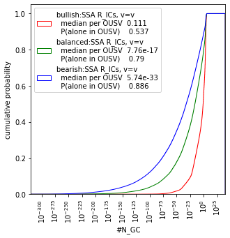
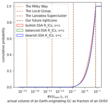
| Simulation behaviour | Updating with observation | Updating with observation |
| AS fixed / HS fixed | 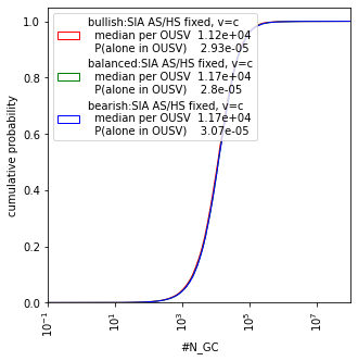 |  |
| HS resource proportional | 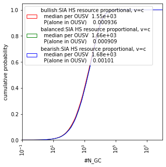 | 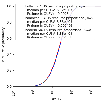 |
| Simulation behaviour | Updating with observation | Updating with observation |
| AS fixed / HS fixed |  | 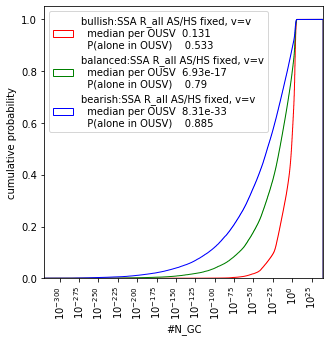 |
Anthropic theory | |||||
| SIA | ADT total utilitarianism | ADT average utilitarianism | SSA | SSA | |
| No XOMs | 1 | 4 | 5 | 6 | 8 |
| HS-fixed | 2 | 4 | 5 | 7 | 8 |
| AS-fixed | 2 | 4 | 5 | 7 | 8 |
| HS-rp | 3 | 4 | 5 | 8 | 8 |
| AS-rp | 4 | 4 | 5 | 5 | 8 |
In the above table, the left column gives the shorthand description of GC simulation-creating behaviour. Equivalent updates have the same colour and number.
| The posterior credence in being alone in the observable universe, conditioned on observation . | ||||||||
| Prior | 1 | 2 | 3 | 4 | 5 | 6 | 7 | 8 |
| Bullish | <0.1% | <0.1% | <0.1% | 0.2% | 70% | 68% | 69% | 64% |
| Balanced | <0.1% | <0.1% | <0.1% | 0.2% | 89% | 89% | 89% | 85% |
| Bearish | <0.1% | <0.1% | <0.1% | 0.2% | 94% | 95% | 95% | 92% |
These results replicate previous findings:
These results fail to replicate Hanson et al.’s (2021) finding that (the implicit use of ) SSA implies the existence of GCs in our future.
To my knowledge, this is the first model that
In the appendix, I also produce variants of updates for different priors: taking (log)uniform priors on all parameters, and varying the prior on .
My preferred approach is to use a non-causal decision theoretic approach, and reason in terms of wagers rather than probabilities.
Within the choice of utility function in finite worlds, forms of total utilitarianism are more appealing to me. However, it seems likely that the world is infinite and that aggregative consequentialism must confront infinitarian paralysis—the problem that in infinite worlds one is ethically indifferent between all actions. Some solutions to infinitarian paralysis require giving up on the maximising nature of total utilitarianism (Bostrom (2011)) and may look more averagist[24]. However, interaction with other GCs - such as through trade - make it plausible that even average utilitarians behave as if GCs are in their future light cone.
Having said this, theoretical questions remain with the use of non-causal decision theories (e.g. comments here on UDT and FDT).
If an Earth-originating GC observes another GC, it will most likely not be for hundreds of millions of years. By this point, one may expect such a civilization to be technologically mature and any considerations related to the existence of aliens redundant. Further, any actions we take now may be unable to influence the far future. Given these concerns, are any of the conclusions action-relevant?
Primarily, I see these results being most important for the design of artificial general intelligence (AGI). It seems likely that humanity will hand off control of the future, inadvertently or by design, to an AGI. Some aspects of an AGI humanity builds may be locked-in, such as its values, decision theory or commitments it chooses to make.
Given this lock-in, altruists concerned with influencing the far future may be able to influence the design of AGI systems to reduce the chance of conflict between this AGI and other GCs (presumably also controlled by AGI systems). Clifton (2020) outlines avenues to reduce cooperation failures such as conflict.
Bostrom (2003) gives a lower bound of biological human lives lost per second of delayed colonization, due to the finite lifetimes of stars. This estimate further does not include stars that become impossible for a human civilization due to the expansion of the universe.
The existence of GCs in our future light cone may strengthen or weaken this consideration. If GCs are aligned with our values, then even if a GC never emerges from Earth, the cosmic commons may still be put to good use. This does not apply when using SSA or a non-causal decision theory with average utilitarianism, which expect that only a human GC can reach much of our future light cone.
The results have clear implications for the search for extraterrestrial intelligence (SETI).
One key result is the strong update against the habitability of planets around red dwarfs. For the self-sampling assumption or a non-causal decision theoretic approach with average utilitarianism, there is great value of information on learning whether such planets are in fact suitable for advanced life: if they are, SSA strongly endorses the existence of GCs in our future light cone, as discussed in the appendix. SIA, or a non-causal decision theoretic approach with total utilitarianism, is confident in the existence of GCs in our future light cone regardless of the habitability of red dwarfs.
The model also informs the probability of success of SETI for ICs in our past lightcone. Such ICs may not be visible to us now if they were too quiet for us to notice or did not persist for a long time.
Barnett (2022) discusses and gives an admittedly “non-robust” estimate of “0.1-0.2% chance that SETI will directly cause human extinction in the next 1000 years”.
I consider the implied posterior distribution on the probability of a GC becoming observable in the next thousand years. The (causal) existential risk from GCs is strictly smaller than the probability that light reaches us from at least one GC, since the former entails the latter.

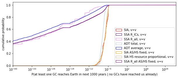
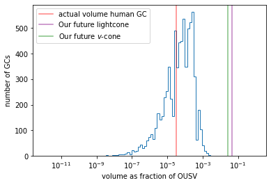
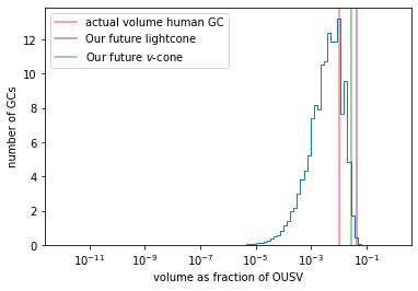
The posteriors imply a relatively negligible chance of contact (observation or visitation) with GCs in the next 1,000 years even for SIA.
However, it seems that the risk in the next is then more likely to come from GCs that are already potentially observable that we have just not yet observed - perhaps more advanced telescopes will reveal such GCs.
I list some further directions this work could be taken. All the calculations can be found here.
I have not updated on all the evidence available. Further evidence one could update on includes:
Modelling assumptions can be improved:
More variations of the updates could be considered:
More thought could be put into the prior selection (though the main results still follow from (log)uniform priors):
I would like to thank Daniel Kokotajlo for his supervision and guidance. I’d also like to thank Emery Cooper for comments and corrections on an early draft, and Lukas Finnveden and Robin Hanson for comments on a later draft. The project has benefited from conversations with Megan Kinniment, Euan McClean, Nicholas Goldowsky-Dill, Francis Priestland and Tom Barnes. I'm also grateful to Nuño Sempere and Daniel Eth for corrections on the Effective Altruism Forum. Any errors remain my own.
This project started during Center on Long-Term Risk’s Summer Research Fellowship.
| The number of hard try-try steps | |
| The geometric mean of the hard steps (“hardness”) | |
| The sum of the delay and fuse steps, strictly less than Earth’s habitable duration. | |
| The probability of passing through all try-once steps in the development of an IC | |
| The maximum duration a planet can be habitable for | |
| The decay power of gamma ray bursts | |
| The average comoving speed of expansion of GCs | |
| The fraction of ICs that become GCs |
| IC | Intelligent civilization |
| XIC | Intelligent civilizations similar to human civilization in that
|
| GC | Grabby civilization |
| OM | Observer moment |
| OUSV | Observable universe size volume |
| AUSV | Affectable universe size volume |
| SIA | Self-indication assumption |
| SSA | Self-sampling assumption |
| ADT | Anthropic decision theory |
| , , | The number of ICs/XICs/GCs that would appear, supposing no preclusion, per OUSV |
| , , | The number of ICs/XICs/GCs that actually appear per OUSV |
| The observation of being in an XIC that has not observed any GCs | |
| The observation of being in an XIC that is not inside a GC | |
| AS | Ancestor simulations; simulations created by a GC of their own IC origins (or slight variants) |
| HS | Historical simulations; simulations created by a GC to be representative of IC origins |
| The probability density function of IC arrival times, excluding any preclusion by GCs. | |
| The probability density function of IC arrival times that do not observe any GCs. | |
| The fraction of an OUSV unsaturated by GCs at time | |
| The comoving volume of a sphere/GC expanding from time at with speed | |
| The actual volume of a sphere/GC expanding from time b at t with speed v which considers the expansion of GCs | |
| The rate of habitable star formation normalised to have integral 1 | |
| The fraction of terrestrial planets that are habitable for at most Gy | |
| The number of terrestrial planets per OUSV that are potentially habitable | |
| The fraction of potentially habitable planet habitable to advanced life at time | |
| The (cosmic) scale factor |
Ade, P. A., Aghanim, N., Arnaud, M., Ashdown, M., Aumont, J., Baccigalupi, C., ... & Matarrese, S. (2016). Planck 2015 results-xiii. cosmological parameters. Astronomy & Astrophysics, 594, A13.
Armstrong, S. (2011). Anthropic decision theory. arXiv preprint arXiv:1110.6437.
Armstrong, S., & Sandberg, A. (2013). Eternity in six hours: Intergalactic spreading of intelligent life and sharpening the Fermi paradox. Acta Astronautica, 89, 1-13.
Barnett, M. (2022). My current thoughts on the risks from SETI https://www.lesswrong.com/posts/DWHkxqX4t79aThDkg/my-current-thoughts-on-the-risks-from-seti#Strategies_for_mitigating_SETI_risk
Bostrom, N. (2003). Are we living in a computer simulation?. The philosophical quarterly, 53(211), 243-255.
Bostrom, N. (2003). Astronomical waste: The opportunity cost of delayed technological development. Utilitas, 15(3), 308-314.
Bostrom, N. (2011). Infinite ethics. Analysis and Metaphysics, (10), 9-59.
Carter, B. (1983). The anthropic principle and its implications for biological evolution. Philosophical Transactions of the Royal Society of London. Series A, Mathematical and Physical Sciences, 310(1512), 347-363.
Carter, B. (2008). Five-or six-step scenario for evolution?. International Journal of Astrobiology, 7(2), 177-182.
Clifton, J. (2020) Cooperation, Conflict, and Transformative Artificial Intelligence: A Research Agenda. https://longtermrisk.org/files/Cooperation-Conflict-and-Transformative-Artificial-Intelligence-A-Research-Agenda.pdf
Eth, D. (2021) Great-Filter Hard-Step Math, Explained Intuitively. https://www.lesswrong.com/posts/JdjxcmwM84vqpGHhn/great-filter-hard-step-math-explained-intuitively
Finnveden, L. (2019) Quantifying anthropic effects on the Fermi paradox https://forum.effectivealtruism.org/posts/9p52yqrmhossG2h3r/quantifying-anthropic-effects-on-the-fermi-paradox
Grace, K. (2010). SIA doomsday: The filter is ahead https://meteuphoric.com/2010/03/23/sia-doomsday-the-filter-is-ahead/
Greaves, H. (2017). Population axiology. Philosophy Compass, 12(11), e12442.
Griffith, R. L., Wright, J. T., Maldonado, J., Povich, M. S., Sigurđsson, S., & Mullan, B. (2015). The Ĝ infrared search for extraterrestrial civilizations with large energy supplies. III. The reddest extended sources in WISE. The Astrophysical Journal Supplement Series, 217(2), 25.
Hanson, R., Martin, D., McCarter, C., & Paulson, J. (2021). If Loud Aliens Explain Human Earliness, Quiet Aliens Are Also Rare. The Astrophysical Journal, 922(2), 182.
Haqq-Misra, J., Kopparapu, R. K., & Wolf, E. T. (2018). Why do we find ourselves around a yellow star instead of a red star?. International Journal of Astrobiology, 17(1), 77-86.
Loeb, A. (2014). The habitable epoch of the early Universe. International Journal of Astrobiology, 13(4), 337-339.
Maartens, R. (2011). Is the Universe homogeneous?. Philosophical Transactions of the Royal Society A: Mathematical, Physical and Engineering Sciences, 369(1957), 5115-5137.
MacAskill, M., Bykvist, K., & Ord, T. (2020). Moral uncertainty (p. 240). Oxford University Press.
Olson, S. J. (2015). Homogeneous cosmology with aggressively expanding civilizations. Classical and Quantum Gravity, 32(21), 215025.
Olson, S. J. (2020). On the Likelihood of Observing Extragalactic Civilizations: Predictions from the Self-Indication Assumption. arXiv preprint arXiv:2002.08194.
Olson, S. J., & Ord, T. (2021). Implications of a search for intergalactic civilizations on prior estimates of human survival and travel speed. arXiv preprint arXiv:2106.13348.
Omohundro, S. M. (2008, February). The basic AI drives. In AGI (Vol. 171, pp. 483-492).
Oesterheld, C. (2017). Multiverse-wide Cooperation via Correlated Decision Making. https://longtermrisk.org/multiverse-wide-cooperation-via-correlated-decision-making/
Ord, T. (2021). The edges of our universe. arXiv preprint arXiv:2104.01191.
Ozaki, K., & Reinhard, C. T. (2021). The future lifespan of Earth’s oxygenated atmosphere. Nature Geoscience, 14(3), 138-142.
Pearce, B. K., Tupper, A. S., Pudritz, R. E., & Higgs, P. G. (2018). Constraining the time interval for the origin of life on Earth. Astrobiology, 18(3), 343-364.
Russell, S. (2021). Human-compatible artificial intelligence. In Human-Like Machine Intelligence (pp. 3-23). Oxford: Oxford University Press.
Saadeh, D., Feeney, S. M., Pontzen, A., Peiris, H. V., & McEwen, J. D. (2016). How isotropic is the Universe?. Physical review letters, 117(13), 131302.
Sandberg, A., Drexler, E., & Ord, T. (2018). Dissolving the Fermi paradox. arXiv preprint arXiv:1806.02404.
Sloan, D., Alves Batista, R., & Loeb, A. (2017). The resilience of life to astrophysical events. Scientific reports, 7(1), 1-5.
Tegmark, M. (2007). The multiverse hierarchy. Universe or multiverse, 99-125.
Tomasik, B. (2016). How the Simulation Argument Dampens Future Fanaticism.
Zackrisson, E., Calissendorff, P., González, J., Benson, A., Johansen, A., & Janson, M. (2016). Terrestrial planets across space and time. The Astrophysical Journal, 833(2), 214.
I discuss how using the remaining habitable time on Earth to update on the number of hard steps n is implicitly an anthropic update. In particular I discuss it in the context of Hanson et al. (2021) (henceforth “they” and “their”). They later perform another anthropic update, using a different reference class, which I see as problematic.
Their prior on is derived by using the self-sampling assumption with the reference class of observers on planets habitable for ~5 Gy (the same as Earth). I write for this reference class. Throughout, I ignore delay steps, and include only hard try-try steps.
They argue (as I see correctly) that to be most typical within this reference class, and observe that Earth is habitable for another ~1 Gy, we update towards . The SSA likelihood ratio when updating on our appearance time alone (ignoring preclusion by GCs) is
where is the Gamma distribution PDF with shape and scale . I take . This likelihood ratio is largest for . We could further condition on the time that life first appeared, but this is not necessary to illustrate the point.

While their prior on n relies on this small reference class, their main argument relies on a larger reference class of all intelligent civilizations, . They use this to model humanity’s birth rank as uniform in the appearance times of all advanced life, not just those habitable for ~5 Gy.
If we use the smaller reference class Gy throughout, then one updates towards , but human civilization is no longer particularly early since all life on planets habitable for ~5 Gy appears in the next ~50 Gy due to the end of star formation. The existence of GCs will have less explanatory power in this case.
If one uses the larger reference class , when updating on human civilization’s appearance time alone (ignoring preclusion by GCs), the SSA likelihood ratio is
Where is the maximum habitable duration, and is the 'number' of planets habitable for Gy.
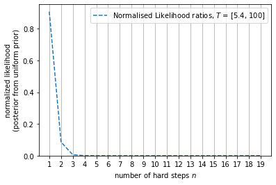
If we believe to be large, then the likelihood ratio is maximum at and is decreasing in : if advanced life is hard then it will appear more often on planets where it has longer to evolve and increasing n makes life harder, so decreases the total amount of advanced life and increases the fraction of life on longer habitable planets. The reference class converges to when decreasing to 5 Gy, and one updates towards .
To summarise, the following are ‘compatible’
Hanson et al. write
If life on Earth had to achieve n “hard steps” to reach humanity’s level, then the chance of this event rose as time to the n-th power. Integrating this over habitable star formation and planet lifetime distributions predicts >99% of advanced life appears after today, unless n < 3 and max planet duration <50Gyr. That is, we seem early.
That is, to be early in the reference class of advanced life, , we require large and large which we have shown are incompatible.
The SSA , SSA and ADT average updates are sensitive to the lower bound on the prior for . When there are no GCs (that can preclude ICs), human civilization’s typicality is primarily determined by : the smaller the more typical human civilization is. If is certainly high, worlds with GCs that preclude ICs are relatively more appealing to SSA.
Here I show updates for variants on the prior for , and otherwise using the balanced prior. Notably, even when which has , SSA gives around 58% credence on being alone, and has posterior . As seen below, increasing the lower bound on the prior of increases the posterior implied rate of GCs.
| Implied posterior on | Posterior on | |
| SSA | 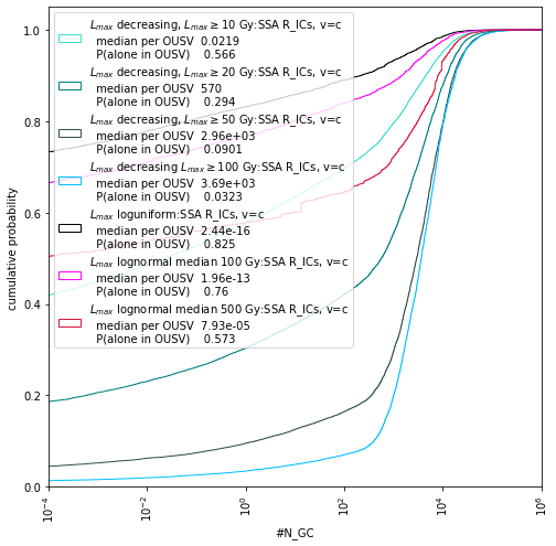 | 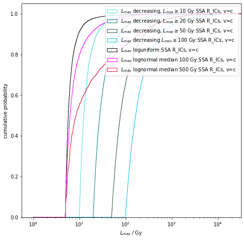 |
| SSA |  |  |
| ADT average | 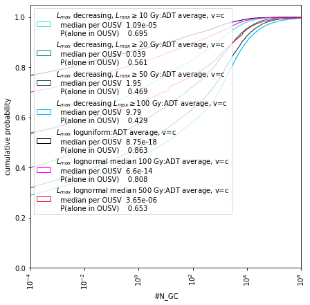 |  |
The following tables show the marginalised posteriors for all updates (excluding the trade and conflict scenarios).
 |  |
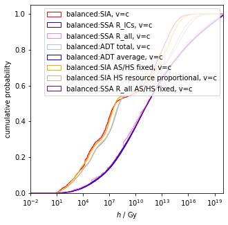 |  |
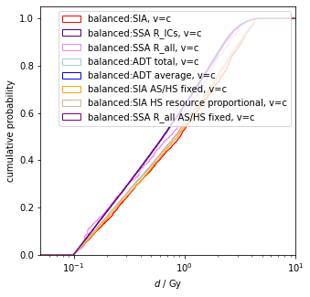 |  |
 |  |
 |  |
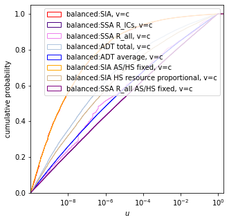 | 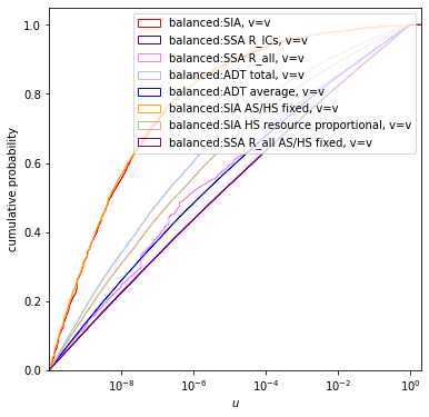 |
 |  |
 |  |
I show that the results follow when taking uniform/loguniform priors on the model parameters as follows:
Which give the following distributions on #NGC
 |  |
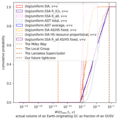 |  |
 | 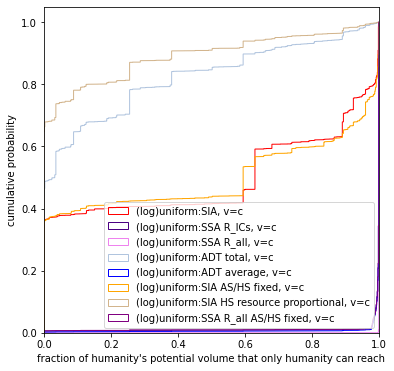 |
 |  |
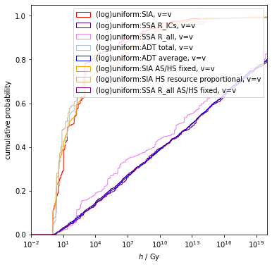 |  |
 |  |
 | 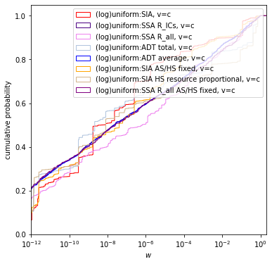 |
 |  |
 | 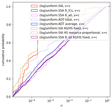 |
 | 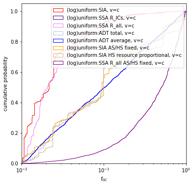 |
 |  |
This takes the same (log)uniform priors, but with . The SSA implied posterior on being alone in the OUSV is now just 59% from observation , and 40% from .
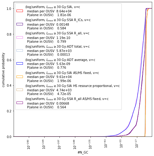 |  |
Currently in this Google Doc. Will be added to this post soon.
Technologies to produce false vacuum decay or other highly destructive technologies will have a non-zero rate of ‘detonation’. Such technologies could be used accidentally, or deliberately as a scorched Earth policy during conflict between GCs. Non-gravitationally bound volumes of the universe will become causally separated by ~200 Gy, after which GCs are safe from light speed decay.
The model presented can be used to estimate the fraction of OUSVs consumed by such decay bubbles. I write for the fraction of ICs that trigger a vacuum decay some time shortly after they become an IC. More relevantly, one may consider vacuum decay events being triggered when GCs meet one another.
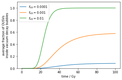
Of course, this is highly speculative, but suggestive that such considerations may change the behaviour of GCs before the era of causal separation. For example, risk averse or pure time discounting GCs may trade off some expansion for creation of utility.
One could run the entire model with replaced by . SSA supports the existence of GCs for and so would similarly support the existence of ICs that trigger false vacuum decay as a deadline.
As mentioned, I model the completion time of hard steps with the Gamma distribution, which has PDF
When , and so . That is, when the steps are sufficiently hard, the probability of completion grows as a polynomial in . Increasing leads to a greater ‘clumping’ of completions near the end of the possible time available.
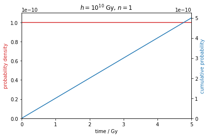
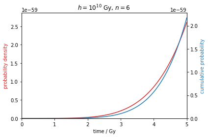
When hard steps are present, it also means that longer habitable planets will see a greater fraction of life than shorter lived planets. For example, a planet habitable for 50 Gy will have approximately greater probability of life appearing than a planet habitable for 5 Gy.
For anthropic theories that update towards worlds where observers like us are more typical -- such as the self-sampling assumption -- increasing while allowing longer-lived planets makes observers like us less typical.
With either the reference class of observers in intelligent civilizations, or all existing observers
This probability is conditional on the fact that there are no GCs for us to see already. The true number is then much higher if one believes that we might just not have seen some already visible GCs.
As our cosmological horizon is increasing, I fix the definition to be the volume of observable universe now
A fuse step is one that has a completion time similar to the completion time of a burning fuse. The completion time could be modelled with a (truncated) normal distribution with small standard deviation and mean greater than zero.
I show the validity of this approximation in the appendix
$\bar{L}$ in Hanson et al. (2021)
$L_{max}$ is used to upper bound the distribution of habitable planets, so could be better thought of as the 99th percentile (say) of the distribution of habitable durations.
I’d recommend Stuart Armstrong’s post Anthropics: different probabilities, different questions for discussion on this point
This assumes that the cosmic zoo hypothesis is false
This is $1/R$ in Hanson et al. (2021)
Forgive the tautological notation
To avoid problems with infinite observers, I consider only observers within the large finite volume (LFV). Strictly, I am using SIA with the reference class of observers within this LFV. If the LFV is large enough, we get the density of XOMs in the Level I multiverse due to its repeating nature. This is similar to the approach discussed here.
Originally referred to as SSA+SIA by Bostrom
Bostrom (2002) gives this as the strong self-sampling assumption.
Strictly, one can use a larger reference class that includes non-actual (merely possible OMs) - this reference class gives SIA
I take $t_L$ = 200 Gy, though in most cases GCs' expansion finishes sooner
The distribution has almost all probability mass on 'no GCs will reach the volumes that a human civilization could expand into'
This assumes that the probability a GC emerges from Earth is equal to the average fraction of ICs that become GCs.
When using SSA $R_{min}$ my prior credence in worlds with zero copies of me is zero (and so have zero decision worthiness by both the first term and also the second term). When taking a fully updateless approach, worlds that contain zero copies of me are given zero decision worthiness by the second term alone, even though I keep a non-zero prior in the world.
Taking $\# V(t_{now}, t_L, v}$ in units of AUSVs
Though using a non-causal decision theory, gains through trade may be possible with GCs outside the affectable universe (e.g. Oesterheld (2017))
This volume itself may be too large: one may instead consider the volume that we can receive a broadcast to and hear back from
The following constants, which wash out in normalisation, are not considered: (a) the average number of OMs per IC (b) the number of AS (on average) created by GCs when the number is ‘fixed’ (c) the number of OMs in created by GCs per fraction of OUSV they control (d) the number of OMs created per fraction of an OUSV given to creating AS or HS
For example, one may choose to use the ratio of resources of agents with my values, to all agents as a proxy of value to disvalue

Hi, thanks so much for this. I don't think I understand it (yet), but it broadly looks like pretty impressive and cool work!
I think its hard for alot of people to understand it lol