Thanks to Arepo, David Thorstadt, Zeshen, and Michael st Jules for looking over this article. Disclaimer: I am not a subject matter expert and this is not a rigorous scientific article. This post is entirely human-written.

Introduction

In a previous article, I wrote a general introduction to the optimizer’s curse, the phenomenon where a combination of random errors and ranking of causes results in the overestimation of top causes and a biasing of results towards uncertain causes. In that article, I mainly focussed on areas such as global health charities, where estimates or errors can be derived from the results of reasonably strong empirical evidence such as randomised control trials.

In this post, I want to explore how the optimizer’s curse might affect tasks that are in the domain of extreme uncertainty. Specifically, I will try and model how the curse could manifest in the ranking of estimates of existential risk, a subject where empirical evidence is thin and experts disagree by orders of magnitude.

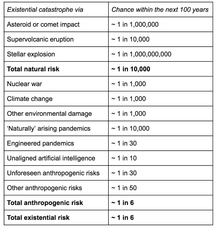
A standard way of ranking existential threats is to take a bunch of threats that have been raised as potentially deadly to humanity, and then for each one of them, to estimate a probability of them destroying humanity. For example, here is a summary of Toby Ord’s estimates from his book “the precipice”:

In this article, I will show you a simple model to simulate the process of ranking threats. I will show that, under a set of reasonable assumptions and input parameters, that the optimizer’s curse will cause such a ranking to overestimate the probability of the top threat by a median factor of more than 50,000. This estimate is highly uncertain, and could be orders of magnitude higher or lower, but in most ranges I looked at the curse would result in multiple order of magnitude overestimates. If this model is anywhere close to correct, then the process of ranking existential threats may turn out to be a machine for vastly overestimating the existential threat to humanity.

In this article I will start with a simple argument for why the process of ranking existential threats could result in drastic distortions due to the optimizer’s curse. I will follow this with a very detailed breakdown of my simple optimizer’s curse model. I will follow that with an exploration of how robust the results are to the assumptions and parameters going into the model, some caveats to the model, and a response to some potential counterarguments, followed by a conclusion.

I recognise that this article is very long. Feel free to skip any sections that bore you: I’m a blogger, not your boss. My goal is to make the model as transparent and easy to replicate as possible, so that others may check it, suggest improvements, or build on it. The code used is here.

Even if this argument is true, and extinction risk is much smaller than previously thought, it does not mean that the threats discussed here should be ignored. A threat doesn’t have to kill all of humanity to be worth preventing, and I will sleep easier at night knowing that smart people are out there trying to prevent bioterrorism, nuclear attacks, and other serious threats.

And lastly: This is a blog article, not a peer reviewed scientific article. Do not blindly trust me, or any other blog: think critically about the arguments I am putting forward. In this article I suggest several ways in which my conclusion could be wrong, and I’m sure others will be able to come up with more. I welcome any rebuttals or improvements, although I probably don’t want to work much more on this subject myself.

The basic case

This is going to be a very long article involving a lot of detail and mathematical modelling. I worry that as a result of this, people might assume that only people using complicated mathematical models have to worry about it. I do not believe that this is true.

The argument I will make is a straightforward extension of the Optimizer’s curse (sometimes called the Winners curse), a well established mathematical phenomenon which I covered in detail in two previous articles here and here. It’s common to a variety of fields, as an example there is an article about how to compensate for the winners curse in genetic association studies. The chief requirement of the curse is that you make rank multiple estimates of some metric, and that those estimates have some error in them which could result in an erroneous overestimate. The method by which you make those errors is not important: it could be due to statistical outliers or due to you making the numbers up.

Here is a very basic 3-step version of the argument as applied to existential risk:

1. Estimating the probability of existential threats is extremely difficult and uncertain, so when you make such an estimation, there’s a chance you will make a large order of magnitude error.
2. If you look at several threats and rank them, then the “lucky” threats which you have overestimated will tend to jump ahead of “unlucky” threats which you have underestimated.
3. Therefore, it is likely that the threat that ranks the highest on your list will be overestimated by a large amount.

In some previous posts here and here, I spent a lot of time arguing for proposition 1, about the large uncertainty in x-risk estimates. In this post, I will argue that propositions 2 and 3 are also likely to be correct.

To make it clear how the “jump” in proposition 2 occurs, I made a very simple illustration involving a threat evaluator looking at two different potential threats to humanity, threat A and threat B:

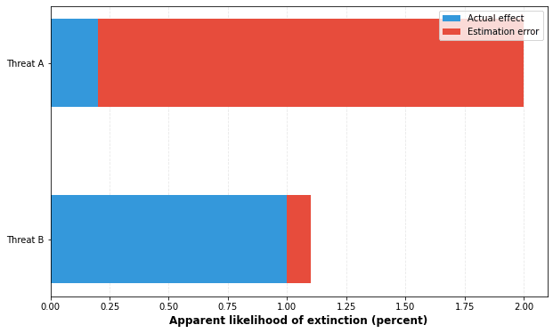
In the above graph the blue bar shows the actual probability of the threat.^[1] In reality, threat B’s probability of causing extinction is 1%, which is more dangerous than threat A, with a probability of 0.25%.

The red bar shows the error that comes from fallible estimators making mistakes. In this case, when estimating the threat from threat A, they have made about an order of magnitude overestimate, jumping their estimate by a factor of 8 to 2%. Meanwhile their estimate of threat B is fairly accurate, at 1.1%.

As a result of this error, It looks like threat A is the biggest threat to humanity, rather than threat B. But the reason it appears to be the top threat is due to the big estimation error pushing it up. In reality the evaluators have overestimated its risk by a factor of 8.

The more likely it is for a large jump like this to occur, the more likely it is that your top cause is a large overestimate. This is true even if you correctly picked the top threat. Because if you had underestimated the top threat, there would be a good chance that another threat would have overtaken it. In my model, sometimes the top threat is correctly chosen, but it does so because an overestimate was made in its favour.

We can also see that threats with high estimation errors are unjustly rewarded in the ranking. The only way that threat B could have competed with threat A’s large overestimate is if we also made a large error estimating it as well. This has implications for existential risk, in that causes with a higher evidentiary basis such as asteroid strikes or nuclear war may end up unfairly disadvantaged compared to more speculative threats, like alien invasion or AI-caused extinction.

I think this argument in this section is strong enough on its own to be worth concern and investigation. However, what I’ve said so far won’t be enough to estimate the magnitude of the effect, or to get a feel for what conditions trigger a large effect. The rest of this article will involve building a simple model that will allow us to get a better feel for the problem, and then interrogating that model.

Part 1: Building a model

Our simple model is going to involve a simulation of an effective altruist threat evaluator, who examines various different threats and ranks them on their existential risk probabilities. This requires some way of modelling both the actual distribution of threats in reality, and the distribution of error in threat evaluators.

Step 1: We pick out a potential threat

So, let’s pretend we are a concerned researcher looking to evaluate potential threats. We live on planet “Idealia”, where everything can be neatly modelled with neat statistical functions.

Our researcher will evaluate threats one-by-one. For example, they may hear about something called “mirror bacteria”, and want to know whether it is a serious cause for concern. We have to model what happens when you pick out a “random” threat like this: what is the distribution of “true” dangers?

Given the high uncertainty from practical surveys (see the next section), it it is very very difficult to figure out the distribution of “true” threats. With grounded interventions, we have meta-analysies and studies to point to. In x-risk estimation, we can only point to estimates, which come after the effects of error have been added on. Human extinction has never happened before, so there is no way to easily validate our models here.

But since I have to pick something for the model to work I think the best choice here is a power law distribution. I have a previous post discussing these distributions in detail. This is probability distribution function where the probability density at some value x is inversely proportional to x:

$p\left(x\right)\propto 1/\left(x^a\right)$

The constant here is incredibly important, as it defines how rapidly extreme values will drop off in likelihood. If your value x (say, the population of a given city in your sample) increases by a factor of 10, this formula says that the probability density of finding that value will drop by a factor of 10^alpha. For example if alpha is 2, it will become 100 times less likely, if alpha is 3 it will become a 1000 times less likely. This will show up as a straight line if you graph the phenomenon such that both axes are logarithmic (a log-log curve).

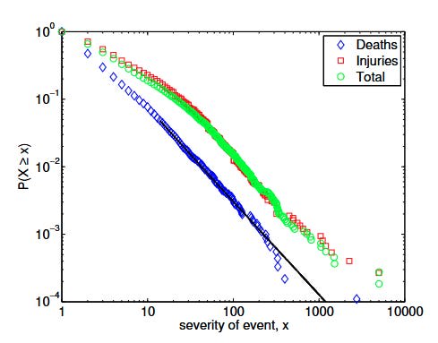
For convenience sake, it’s generally easier to plot this as a cumulative distribution function, which tells you the probability that a random event is greater than a value x. On a log-log curve, this will also show a straight line on a log-log curve, with a slope of alpha-1. As an example, the following graph shows the power-law behaviour in the phenomenon of deaths from terrorist attacks, which produces a log-log straight line over roughly 3 orders of magnitude:

The reason that this is a natural choice to model our threat distribution is that a wide variety of measures of danger exhibit power law behaviour. The following is a list of some of the danger metrics that can be approximated with power laws over some range (see my previous article for the details):

earthquake magnitude, moon crater diameters, solar flare intensity, war deaths, asteroid impact energy, earthquakes, topographic depressions, sinkholes, tropical cyclones, rain cluster areas, rain total precipitation, terrorist attack deaths, flood intensity, and wildfires.

The logic for modelling existential threats with power laws thus goes like this:

1. A significant number of danger metrics follow power law distributions.
2. “Probability of causing extinction” is a danger metric.
3. Therefore, the power law distribution is a reasonable choice for modelling x-risk probability distributions

To be clear, this is not a super strong argument. As I covered in the last post, the phenomenon above very often only exhibits power law behaviour over certain ranges, often breaking at values below or above a certain range. And many phenomena which appear to be power laws are actually different distributions which just happen to look like power laws over a zoomed in range of values.

Another important point against the argument is that these trends are seen within threat areas, where we are comparing the frequency of small earthquakes to big earthquakes and the frequency of small asteroids to big asteroids. Here, we are trying to model the threat between different cause areas, comparing the overall danger of asteroids to the overall threat of nuclear war, etc. There is some reassurance with the trend for terrorist attacks, which still seems to hold to power laws even though terrorist attacks can be conducted by different people in a variety of different ways.

So I want to be clear that this is necessarily a flawed approximation. However, given that we have absolutely zero data on the actual frequency of global human extinction, and that getting one more datapoint on the matter would be the end of humanity, we’re just gonna have to go with it, and heavily explore the consequences of various assumptions around it.

One thing to note about the power law is that it is very long-tailed (drops off less at higher values), compared to other statistical patterns seen in nature. Compare the following graphs of a normal, log-normal, and power-law distribution:

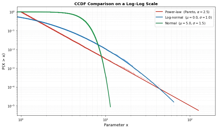
The power law distribution drops off much slower over long ranges. Why is this important? Well, as I discussed in a previous post, the more long tailed a distribution is, the less pronounced the optimizer’s curse tends to be, because there is a greater distance between the actual probability of two neighbouring samples, making it harder to jump the gap with an error. This means that if we still see the optimizer’s curse in a power-law model (which, spoiler, we will), then deviations from the power law distribution will probably make the curse worse, rather than better. In this paper, researchers looked closely at 15 natural phenomena which appeared to show power law behaviour, and found that 2 held up as power-laws and one as a double power law, with the rest being either inconclusive or falling off at higher values. So while the power law is not the upper limit for long-tailedness or anything, it does seem like the choice is on the balance favourable to the “no optimizer curse” side.

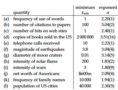
The last reason to choose the power-law distribution is that it’s simple and convenient to play around with. There are only two parameters, alpha and a scaling factor xmin, and the latter has no effect on the optimizer’s curse. Furthermore, the alpha exponent generally has a limited range of values in natural phenomena. We can see in the following table from this paper that alpha is roughly between 2 and 3 for a wide variety of phenomena:

This makes it convenient to explore the range of alpha values, as we will do so in detail later.

The power law can be created by sampling from the following function, where u is a random value between 0 and 1:

$P=Xmin(1-u{)}^{(-1/\alpha )}$

Where u is a random number between 0 and 1.

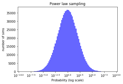
The x_min here represents the cutoff for inclusion: we are assuming that threats that are less than 10^-7 are dismissed as trivial.

We can see that on a log-log scale with logarithmic binning, this produces a straight line, as we would expect:

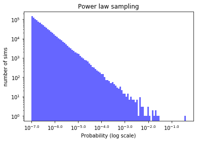
This means that probability values that are 10 times higher are 10 times common. So if our threat rating organisation is picking out a threat at random, it’s orders of magnitude more likely to be a threat with actual probability 1 in a million than an actual threat of probability 1 in a 100.

We pick out an alpha of 2, at the lower, more dangerous end of the typical 2-3 range for alpha discussed in the previous section. The xmin scaling factor is arbitrarily set at 10^-7: this value does not affect the optimizers curse magnitude for the range we are exploring here. It was chosen to make the top “actual threat” in our simulation appear to be roughly 1 in a 100 chance, but could be set to anything.

Step 2: We make mistakes

Our hypothetical researcher is fallible. If the actual threat of mirror bacteria is 1 in a million, there’s no guarantee that the researcher will correctly guess this. How much error are they likely to make in their estimates?

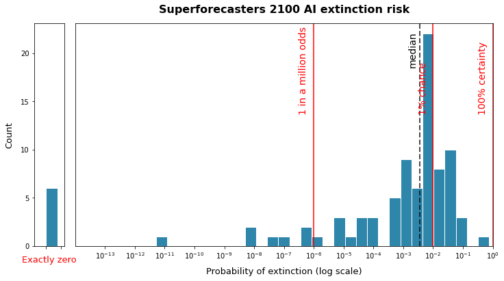
In a previous article, I looked at this question in depth, using evidence from various expert surveys. The spread of answers between experts could differ substantially: for example, here is the spread of superforecasters on long-term AI-risk:

And on long-term nuclear extinction risk:

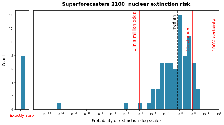
The shapes of this curve varied significantly depending on the group surveyed, the threat being evaluated, and the timescale of the format. I recommend reading through my other post for details.

The important takeaways from this analysis was that x-risk estimates varied by many orders of magnitude within-groups, and a few orders of magnitude between different groups as well. This is also discussing the spread of estimates, not the spread of actual error, which may be larger.

I think from this evidence, we are justified in modelling the error here as multiplicative, rather than additive as was the case in the previous optimizer’s curse article. For a multiplicative error, we will take the real answer, then multiply it or divide it by some error factor.

This matches with the way existential risk is often estimated by multiplying many factors together, as I discussed in this article. There is a natural distribution that arises as a result multiplying several positive factors that each have an independent error, and that is the lognormal distribution. This distribution varies over several orders of magnitude, and looks like a bell curve on a logarithmic scale. It’s not a perfect fit with the distributions shown above, but it should be a good enough approximation for our purposes.

In my simple model, I’m going to be approximating the error by sampling a multiplicative error from a lognormal distribution, centered around a multiplicative factor of 1. Here is an example distribution, with mean of zero and lognormal standard dev of 2:

We simulate the error by sampling an error factor from this lognormal distribution. This error factor will then be multiplied by the actual probability from above to yield the estimated probability for this cause.

The equation is:

10^N(mean, stdev)

Where N is a sample from a normal distribution with the given mean and standard deviation.

The default parameters we will use are a lognormal mean of 0 and a lognormal standard deviation of 2, which I approximate from looking at the spread of estimates by various groups of experts in this post. This corresponds to the assertion that we expect our estimate of each threat to be within plus or minus two orders of magnitude of the correct probability roughly 68% of the time.

This is a simplified model, of course, and the reality is a lot more messy. In particular, there is a problem with this model when the actual probability is very high: it will lead to estimates that are greater than 100%. For example, if the true value is 10%, and you overestimate by a factor of 100, you’d get a value of 1000% probability, which doesn’t make any sense. In our model, we will crudely correct for this by rounding any “estimate” above 100% to exactly 100%.

Step 3: We evaluate lots of different threats and find the “top threat”

Our fictional researcher then expands the analysis, repeating the process above to examine lots of different threats, in order to rank which is the most dangerous, and pick out the top threat.

In our model, we multiply the sampled numbers from step 1 and step 2 together to produce the estimated value, with errors included. We repeat N times to correspond to each threat evaluated.

As default I will set the number of threats N to 100. For reference, in Toby Ord’s book on existential risks, “the precipice”, he published an estimate for ten threats: however, the list was certainly non exhaustive, we have to imagine that there were probably more threats that have been loosely considered but not included in the book. I argue that if a threat like “grey goo” was dismissed based on a back of the envelope calculation or a colleague’s view that it was no longer likely, then it still counts here. In an alternate world, the calculation might have gone the other way, and it would have ended up on the list.

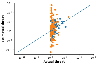
The following graph shows one simulation of the first three steps:

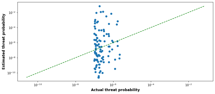
The x-axis shows the actual threat probability for the 100 threats we are looking at (note the log-log scale), while the y-axis shows the estimated threat probability of the corresponding threat. The dotted green line is the line of accuracy, showing where the dots would land if the estimators were perfectly accurate.

We can see that, for these parameters, there is a large difference in actual threat probability between different threats: the top actual threat is over 100 times as dangerous as the lowest threat of the ones investigated.

However, this is dwarfed, for these parameters, by the gargantuan differences in estimated effectiveness, running over 10 orders of magnitude. And in fact, the top apparent threat, according to the estimate, is actually fairly low probability: it just happened to be one that got lucky and was overestimated. Also note that some threats that really are highly dangerous are being underestimated here: in the image above, many of the top actual threats appear to lie in the bottom half of threats when the ranking is done.

The following table shows what the odds of the above pictured run would look like to the researcher, looking just at their top 10 apparent threat probabilities:

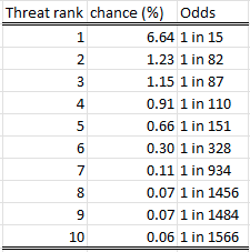
I don’t think estimates like this would look out of place if you posted them on an effective altruist forum. You can compare it to Ord’s list of estimates at the top of this article: they are not identical, but for anthropogenic causes at least,^[2] they’re not that different either. I did help matters along here by deliberately choosing a scaling factor that would peak out at around 5%.

In this case, when our researcher picks the top apparent threat, they believe that the probability is 6.64%, when in reality the threat has a probability of 0.00002%.

Step 4: We repeat and examine the results

There’s a lot of randomness about what happens each time you take 100 threats and evaluate them. The one run looked at in the last step could have been lucky or unlucky. In order to establish trends, we pretend that this is run a lot of different times independently, and analyse the results.

We repeat the process above several thousand times, and graph the results of all the different simulations. First, we will graph the actual probability of the top threat on the same graph as the estimated probability of the top threat:

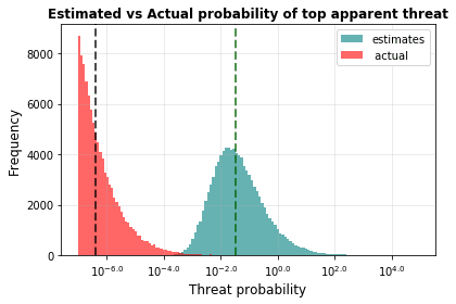
It can be seen that most of the time this simulation is run, the top apparent threat is really somewhere around the 1 in a million probability, but appears to be around 1 in a 100 probability. We can graph the overestimate directly as well:

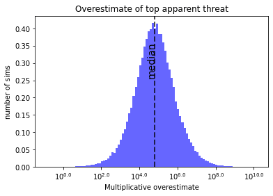
The median result of this methodology is that the top threat value is overestimated by a factor of 60,000.

What does this look like for the threat evaluator? At the end of all their excruciating, detailed, unbiased analysis of a hundred different threats, they might produce a top threat that they believe has roughly a 1% chance of wiping out humanity. But they will be wrong: purely because of the optimizer’s curse, the actual chance of their top apparent threat wiping out humanity will be something like 0.0001%.

Part 2: Interrogating the model

So, I made a model, put in some reasonable seeming parameters, and it spat out a result saying that threat evaluators are boosting their top threats by a gargantuan portion. So what? As I’ve emphasised, the parameters in the model are highly uncertain, and I certainly am not able to ensure that they are precisely accurate.

What we want to do now is evaluate how sensitive the model is to our assumptions, and how robust its conclusions are. So in this section, I will take a look at the key parameters, and evaluate the effect they have on the magnitude of the curse.

I’ll warn that this will be fairly long and involve a large number of graphs, in an attempt to make the assumptions and parameters of the model as transparent and understandable as possible. If you are not interested as much in the details, you have my permission to skip ahead to the later sections.

Parameter 1: Number of threats evaluated

First, we will examine what happens when you expand your search and look at more potential threats. Using the default values described in part 1, I will repeat the whole analysis but change the number of threats we examine in each run. Below is a graph of the resulting overestimate of the top apparent threat with different parameters in place.

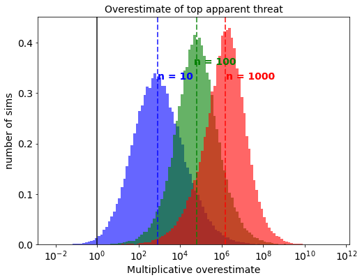
As you increase the number of threats you evaluate, the magnitude of the optimizer’s curse increases. If you just evaluated 10 threats, we get a median overestimate of around 1000x: at 100 the overestimate becomes about 100,000x, and at 1000 threats it jumps even further to a million times overestimate.

This jump happens because the more instances you look at, the more likely you are to really mess up when evaluating a threat, pushing it to the top of your list.

The multiplicative error appears to be roughly proportional to the number of interventions that are investigated. This means that if you put in the effort to 10x the number of threats you have looked at, you should expect this to result in a 10x greater overestimate of your top result.

Does this mean that ranking lots of threats is pointless? Not exactly. If we look at the actual probability of the top apparent threat, it is slightly higher when we look at more threats, indicating that the process hasn’t given us zero information. But the differences in median are pretty small:

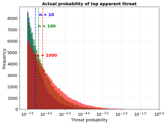
This means that while it looks to the evaluator like the process of evaluating threats is making a big difference and unearthing order of magnitude greater threats, with these parameters it is almost entirely illusory. The actual effect is marginal by comparison.

Parameter 2: Alpha law parameter

We are modelling the “true” value of threats using a power law distribution, which has a crucial “alpha” parameter that determines the drop-off in probability. As a reminder, for every 10 times increase in threat danger, there is a 10^alpha times drop-off in the likelihood of seeing that value of danger.

The key effect of this parameter is that a very low alpha means that there can be quite a large difference in probability between the top actual threat and the next top actual threat, whereas a high alpha means there is not likely to be much. When the gap is small relative to the error, the optimizer’s curse kicks in, when it is large it is diminished.

I have chosen alpha values of 1.5, 2, and 4 to investigate because, as I describe in part 1, most observed power laws in the natural sciences have alpha values between 2 and 3. The results are as follows:

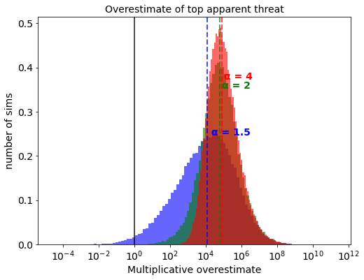
Changing the alpha from 2 to 4 doesn’t have a huge effect on overestimates: we appear to be in a regime where the noise dominates either way. On the other hand, dropping the alpha to 1.5 makes a meaningful, but not super large, difference, as the difference between successive threats in actual terms starts to matter. Dropping further would have a more dramatic effect. Dropping the alpha to 1 results in a divide by zero error.

If we look at the actual probability of the top apparent threat, we can see that when the alpha is 3 essentially all the causes are in a small sliver next to each other anyway, but when alpha is 0.5 we end up getting some actual signal through the noise:

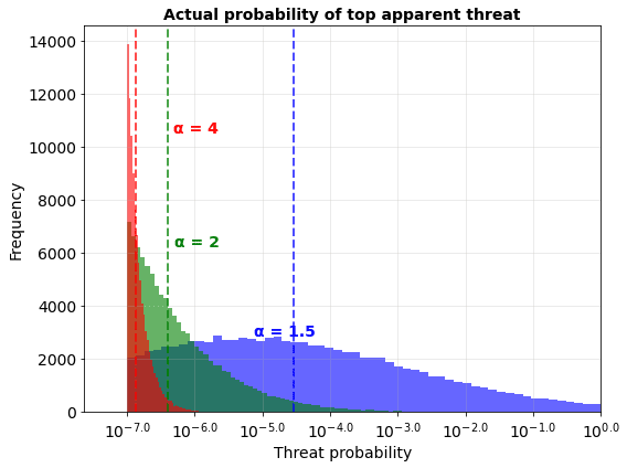
In conclusion, the alpha parameter is very important. The process of ranking existential threats is much, much more useful if the alpha is low, compared to it being high.

Parameter 3: Error lognormal standard deviation

This parameter represents how high the typical error is for each threat that you evaluate. If the lognormal standard deviation is 1 for a group of threats, then you would expect that 68% of the time, your estimate is within 1 order of magnitude of the correct answer. If your standard deviation is 2, then you expect that 68% of the time your answer is within 2 orders of magnitude of the correct answer. Two of my previous posts here and here explain why I would expect this value to be 1 or more.

The default value I use here is 2. The following graph shows what happens if this is varied to 1 or 3:

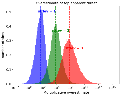
We can see that the more uncertain your estimates (with higher standard deviation), the more you overestimate the top threat. A rough rule of thumb is that the overestimate increases by a factor of 100 for every unit increase in the standard deviation of lognormal error.

The following graph shows how this affects the effectiveness of your ranking strategy, by graphing the actual probability of the top apparent threat:

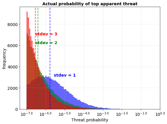
This reveals that you don’t get much improvement from lowering the error from a stdev of 3 to a stdev of 2. In both cases the estimates are simply too noisy to get very useful information out of the ranking process. But improving further to a stdev of 1 does make a real difference. For a stdev of 1 the “true” probability of the highest apparent threat is roughly 10 times higher than the “true” probability of the highest apparent threat in the higher stdev scenarios.

Parameter 4: General optimistic or pessimistic bias

Lastly, we can take a look at the effect of bias. In our default case, we assumed that the error of the estimators was symmetric. This would mean that they were just as likely to overestimate as to underestimate the probability of each threat.

This isn’t necessarily true, however. We could easily imagine a threat evaluator having a generalised optimist or pessimist bias, where they consistently underestimate or overestimate the probability of extinction for all threats. This could be for any number of reasons, such as having misplaced cynicism about humanities ability to work together to end threats.^[3]

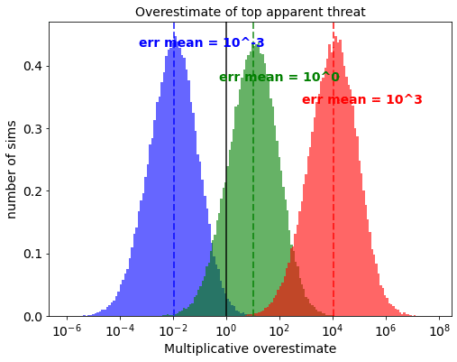
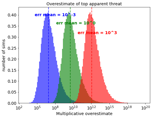
Picture below are the overestimates, that result when the “mean” of the overestimate is varied between an optimistic bias of underestimating every threat by an average factor of 1000 (in blue), to a a pessimistic bias of overestimating every threat by an average factor of 1000 (red). All other parameters are default.

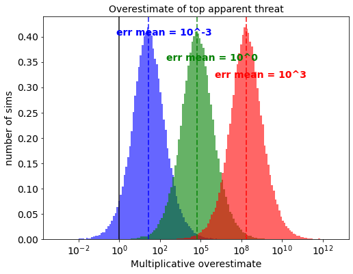
What’s interesting is that even with a large optimistic bias, where the danger of each cause is on average underestimated by a factor of 1000, the ranking process still manages to produce an order of magnitude of overestimation of the top threat. And if the bias goes the opposite way, you could end up with a 100 billion times overestimate.

I don’t want to anchor you with my choice of boundaries for the optimistic or pessimistic bias here. You might believe that x-risk estimators are much more biased or unbiased than 1000x. Biases could also occur in a more complicated way than is modelled here, such as an org being unwilling to give out probabilities lower than 1 in a thousand or above 1 in 10.

I will not show the effect of bias on the actual probabilities of the top apparent threat, because they are all identical. This is because the parameter has zero effect on the actual selection process or the relative odds given to each threat. They could be affected if some subset of threat estimation was biased while others weren’t, but I won’t try and model that here.

Combining factors

So far in this section, in every single case the threat probability of the top cause has been overestimated by an order of magnitude or more.

However, I want to be clear that in the last few sections, I have been only varying one parameter at a time, while keeping everything else at a “default” value. If you combine some of them, you can end up with situations where the optimizer’s curse does not kick in.

IF the alpha is 0.3 AND the number of interventions is 10 AND the stdev is only 1 AND you have a large bias against doom, then you can end up with an underestimate. The following graph is a repeat of the error mean calculation, but with every other parameter set to pessimistic values:

You could also end up with an underestimate or small effect if you push one of these factors far beyond what is shown here, for example if you think the average threat is underestimated by a factor of a million or more.

Of course, we could then go the other way, and see what happens when the alpha is 3 AND the number of interventions is 1000 AND the stdev is 3:

Following all of these extremes results in a top threat estimate that is 1 trillion times too high.

So I do not want to say that it is completely impossible for the optimizer’s curse not to kick in with the model we are using here, but it seems like you have to squeeze the model pretty hard to avoid it. In any typical simulation, using this model, the top charity will be overestimated by orders of magnitude.

Other parameters and Caveats:

I have not considered the effect of correlation between different threat estimates. I explored this topic in a post analysing the regular optimizers curse, with the finding that correlation between actual values raised the magnitude of the curse, but correlation between estimation errors decreased it. Most likely the cumulative effect would be a decrease in curse magnitude.

I did not include the “xmin” factor from the power law equation, as it generally has no effect on the optimizer’s curse magnitude. All it does is shift the actual probabilities higher or lower.

One shortcoming of the model is that under certain circumstances it can spit out actual probabilities or estimated threat probabilities that are higher than 100%, which obviously doesn’t make sense. I have tried to sidestep this by lowering the xmin factor so that this doesn’t happen, but a full accounting would have to consider what happens in these cases. People’s methods of estimation may change as estimates move above the 5% mark, for example, which is not accounted for here.

I explained my reasoning for the model distribution shapes I used above, but they aren’t the only shapes you could choose. The process of making estimates and errors is a lot more complicated than just picking from a defined distribution. The hope is that the simple model captures enough relevant parts of the real process to be informative.

Speculative bias

Next, I want to explore an issue that was important in the regular optimizer’s curse scenario. In that post, I found that the optimizer’s curse could result in a significant bias toward uncertain causes over more grounded ones.

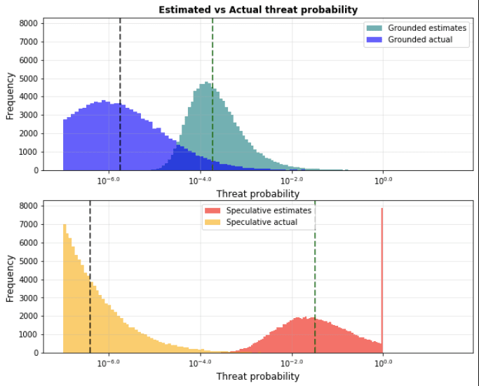
A similar effect occurs when we are looking at ranking existential threats. Let’s say we look at 100 threats, but this time they vary in uncertainty. 50 of them are “grounded”, while 50 are “speculative”.

We will say that grounded and speculative threats are identical in all ways, except that the speculative threats are much more uncertain, with a lognormal standard deviation of 2 orders of magnitude, rather than 1 order of magnitude for the “grounded” threats.

We will plot the actual threat probability against the estimated threat probabilities, with the “grounded” intervention in blue, and the “speculative” intervention in orange:

We can see pretty clearly that the greater spread of the orange threat estimates leads to outliers on both the positive and negative side. But when ranking, we end up only looking at top threats. The blue dots have no chance here! It’s essentially guaranteed that an orange threat will win out.

Let’s look at estimated vs actual threat:after a number of simulations. Here is the result, with “grounded” threats on the top, and the “speculative” threats on the bottom:

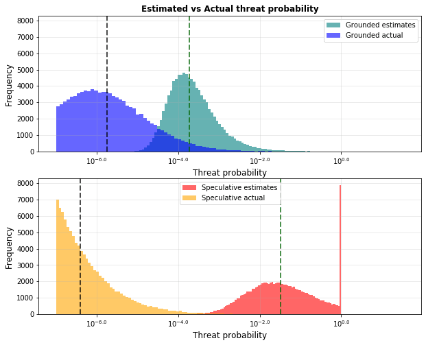
For the median case, the top apparent speculative threat appears 175 times more dangerous than the grounded threat, but in reality, the situation is flipped: the top apparent grounded intervention is actually 4 times more dangerous.

This has interesting implications: for example, when Toby Ord estimated existential risks for his book “the precipice”, he estimated that AI existential risk was 100 times that of nuclear risk. This is less than the 175 times difference from the analysis above! If he also believed that AI risk estimates were significantly more uncertain than nuclear risk estimates, he could still reasonably conclude that nuclear risk was the bigger threat, after compensating for the effect of the optimizer’s curse.^[4]

Part 3: Objections

Once we’ve built a model, and checked its sensitivity to assumptions, we are still not done. Next we want to think critically about the model and its implications, and think about any objections one might have to the model as a whole. In this part, I will go over a few possible objections, some which I don’t find convincing, and some which I think are pretty strong.

Lack of validation:

I think a key shortcoming of this model is that there is no easy way to validate whether it is true or not. Once again, there is no way to know the “true” probability of a threat causing human extinction, because if it actually happened there’d be nobody around to make a retrospective judgement about it.

I have tried to compensate for this by showing that the effect holds up under a wide variety of conditions. Reality doesn’t need to match up exactly with the model I have made here, it just needs to be close enough for the conclusions to follow.

There may be ways to at least partially check the conclusions. If you are running a research group, you could try and find an analogous situation where the “true” probabilities are known, ask them to make rankings, and see if the results match up with the predictions here. I don’t have the time, money, or motivation to do that, but if anyone else wants to, be my guest!

It’s just a model!

One might point out that my model here is simplistic and lacking in empirical grounding, so why should anyone trust it?

Well, if you are concerned about lack of empirical grounding, boy do I have news for you about existential risk estimates!

Whenever anyone makes any existential risk estimation, they are necessarily relying on non-empirical models of the world to some extent. One EA forum post placed “If it’s worth doing, it’s worth doing with made up numbers ” as one of four key norms underpinning EA’s implicit epistemology:

Spend enough time around EAs, and you may come to notice that many EAs have a peculiar penchant for sharing probabilities about all sorts of events, both professionally and socially. Probabilities, for example, of the likelihood of smarter-than-human machines by 2040 (in light of recent developments, Ajeya Cotra’s current best guess is around 50%), the probability of permanent human technological stagnation (Will MacAskill says around 1 in 3), or the chance of human extinction (Toby Ord’s book, The Precipice, ends up at about 1 in 6). 

These numbers are rarely the result of rigorous mathematical modelling, but are more commonly a quantification of ones general intuition about a topic, justified on the grounds that a made up intuitive number still contains some information worth communicating.^[5]

If you want to be skeptical of my uncertain model on the basis of high uncertainty, you should apply similar skepticism to existential risk estimates coming from EA organisations as well.

The power law approximation is a little dodgy, right?

Yep. If my argument turns out to be wrong, I would guess it would be due to something about the power law approximation that I used for the “actual” probability distribution. There’s just not a great way of determining it, so I have picked what I think is the best available option. You can see the justification for the approximation, and the corresponding shortcomings, in the “step 1” discussion in part 1 above. .

You are updating with no information!

If we take this model seriously, it seems to suggest that one should take their top estimate and drop it by several orders of magnitude, based on nothing more than this statistical argument, and not on any arguments that are specific to the threat itself. It might seem crazy to think that you should drop your probability estimates by orders of magnitude, based on seemingly no new information about the actual cause itself.

However, I want to point out that there is new information here. The very fact that the threat came out on top, in an environment with very high uncertainty, is in of itself strong evidence that the threat is overrated.

This is not unprecedented behaviour: when companies make bids on auctions, they deliberately bid lower amounts than they actually believe the thing is worth, to cancel out the effect of the winners curse. The correct move is to bid what you would believe something is worth after being given the information that you won the auction, an indication that other people did not bid as highly as you.

This procedure is merely doing the same thing for probability estimates. The reason it seems so extreme is because the errors themselves are so extreme. When you venture out and try to reason in realms of high uncertainty, you may end up with crazy seeming results.Typically academic fields tend to abandon quantification when confronted with this level of uncertainty, but by plunging forward anyway, you have exposed yourself to correspondingly high levels of risk.

Individual estimates vs group estimates

A lot of the analysis has been focussed on the error of a single researcher acting on their own. One could argue that when you discuss your estimate with different researchers and understand their arguments and research, you will get closer to the truth, counteracting the curse.

This may be true, but to what extent? If you have a threat that you have overestimated by a factor of 50,000, how much do you expect debate and discussion to cut that error down? Even if you update by a factor of 100 in the right direction, you are still 500x off!

There are also problems with group dynamics that can make things worse. The error that led you to overestimate a threat might be present in others as well. People with high P(doom) estimates might have similar beliefs and end up hanging around each other, reinforcing their shared error, and people with low P(doom) beliefs might end up quitting an organisation out of annoyance. The people with high P(doom) beliefs might be more motivated to recruit and spread the word, spreading that belief further.

Is the curse already accounted for?

When I discussed the optimizer’s curse in the context of Givewell, one of the strongest defences they had was that in certain cases they were already compensating for it. For example, when calculating the impact of deworming, Givewell was concerned about the heavy reliance on the outcomes of a single randomised control trial. As a result of this, they included a “replicability adjustment”, which dropped their estimate by a factor of around 8 (see my optimizer’s curse article for more details, or their reasoning for the exact number here).

Now, if deworming estimates get cut by a factor of 8 due to being based on only a single randomised control trial, what does that say about what we should do in cases where an estimate is based on 0 trials of any kind?

I looked, and I was unable to find any reference to existential threat evaluators deweighting extreme results due to a lack of evidence. It’s quite possible I missed something, of course, but as far as I can tell this sort of correction has been totally limited to Givewell evaluations, perhaps due to the mistaken impression that the effect is confined to cases of statistical errors arising from trials.

It’s possible that the lack of evidence has been accounted for in other ways. Perhaps someone who initially guesses a 20% chance of extinction is subtly dropping that down to 5% on the grounds of epistemic modesty. But it’s unlikely they are doing so in the exact right way to counteract the effect of the optimizer’s curse.

Do top threats have extra scrutiny applied?

If you do a lot of trials on the effectiveness of a drug, or the efficacy of a global health intervention, you expect them to eventually converge on the right answer. A drug with positive results from a handful of studies could be a result of p-hacking or luck or other ways of gaming the system, but if you have dozens of high quality studies and metastudies, then we can be pretty damn sure it works. There are large areas of science which we can be very certain of precisely due to the high level of applied empirical scrutiny.

Is debating existential risk likely to lead to the same result?

The best case scenario is something like asteroid risk, where the historical record and physics principles give us decent answers to key aspects of the question. We can get a decent estimate for “what is the chance of an asteroid of X diameter ending up on a collision course with earth”. But even with asteroid risk, we don’t have a reliable estimate of how likely we are to deflect the asteroid. I do not see how any amount of experiments or debate can lead us to a completely accurate answer to the latter question. For something more speculative like AI risk, there are no randomised controlled trials to act as tiebreakers, nor are there any regular trials or empirical experiments that directly test extinction probability.

When it comes to science, we have good reasons to expect extra scrutiny to result in a convergence towards the truth, because we can conduct empirical experiments which have different results for different theories. This is not the case when it comes to existential threat probabilities: instead we are trusting in something like the “marketplace of ideas” to come up with a correct mathematical estimate. I simply do not think this is very reliable.

One experiment from the forecasting research institute actually tested whether debate between groups with different opinions would lead to convergence to some correct view, and found that in general it did not:

“Despite incentives for both persuasive rationales and reciprocal scoring, there was very little convergence within teams during the XPT. That is notable because both incentives might plausibly lead people to change their minds. Well-thought-out rationales might prove more persuasive; reciprocal scoring challenges forecasters to better understand other participants and what they think. Few minds were changed during the XPT, even among the most active participants, despite monetary incentives for persuading others. “

Are you saying that all x-risk research has been useless?

Some, but not all.

I think x-risk researchers have been unsuccessful at the specific question of estimating existential threat probabilities. They may have brought the uncertainty down from “ridiculously, unimaginatively uncertain” to merely “extremely uncertain”, but unfortunately this is not enough to avoid the curse.

But outside of that one specific question, x-risk researchers have done valuable work amassing information about various threats to humanity. We don’t need to know the exact probabilities of catastrophe to take action to prevent danger, and threats do not have to end humanity to be worth protecting against.

The parameters happen to be the ones that minimise the curse!

While I have shown that the curse applies across a wide variety of modelling assumptions, it doesn’t apply in every case. I have shown that there are combinations of parameters where the curse is low to zero. It could be the case that we are in one of these low-curse regimes.

But unless you had previously done this exact analysis yourself, and determined that we were in fact in one of these low-curse regimes, then there is no reason to expect that this is the case. As far as I know, existential risk estimators have not done this.

My cause is special!

As we have seen, the overestimate you would expect to see for each threat is highly dependent on its uncertainty. If you are absolutely certain about your estimate of one threat, then the curse says you should not change your estimate.

I don’t think very many threats warrant this level of certainty. You should be considering not just your uncertainty, but the possibility that you are underestimating your uncertainty. Many factors that lead one to erroneously high estimates will also lead you to erroneously overconfident estimates. I would be especially wary of any confidence that arises from theoretical arguments rather than hard evidence.

The model is incomplete.

It’s true that I left some stuff out. For example, I left out correlation between causes: the effect of this absence is probably to make the curse look worse. I also left out the possibility of the actual distribution being shorter tailed than the power law, as is common in nature. The effect of this absence will make the curse look less bad.

Other than that, there is no reason to be certain that putting more detail will make the curse less bad: it could very well go the other direction. The only way to know for sure is to put more effort into it than I’m willing to do at the moment.

To be clear, I would be utterly delighted if this article sparked a bunch of followup explorations of the various aspects of the problem, and the evidence underlying each of it’s assumptions. I would be disappointed if this article was treated like the end of the story!

Why do different groups have similar rankings?

If you run the model over and over again, usually it will produce a new “winner” each time. But in the field of existential risk studies, a few threats like AI risk, nuclear risk, and biorisk seem to top the list every time, in contradiction to the model. What gives?

I would be more sympathetic about this argument if the existential risk community were not so closely knit and so clearly influenced by each other. I think what has happened is that early estimates of the dangers of threats produced overestimates due to the optimizers curse, which then influenced similar errors and overestimates in later organisations.

There is nothing in the optimizer’s curse analysis that says different groups can’t make the same errors in their rankings.

It’s pretty easy to tell a reasonable story about how, say, AI risk has been overstated. Yudkowsky, considered the founder of AI safety, has always been concerned about existential threats. In 1999 he rated the top threat as “a nanowar”, expected by 2015. In the early 2000’s, he became convinced that AI was the biggest threat, and wrote a chapter in a book called “Global catastrophic risks” on the topic, edited by Nick Bostrom. Yudkowsky founded the Rationalist movement and MIRI, while Bostrom founded the Future of life institute.

When the Effective Altruist movement formed towards the end of the 2000’s, it was heavily embraced by the rationalist movement, and there was extensive intermingling within the groups that continues to this day. Initially focussed on global health, EA over time became the most influential group working on existential risk discussion, including works such as Toby Ord’s “the precipice” in 2020 which ranked existential risks. Toby Ord had previously worked alongside Nick Bostrom at future of life institute from 2014-2019.

With this (highly condensed) history in mind, it’s not difficult to come up with a story about what happened here. AI safety arguments were floating around more than a decade before EA started making their official existential risk rankings. The EA community was primed through selection and founder effects to overestimate certain existential risks as a result of its ties to the rationalist movement. As the most influential group in existential risk studies, EA’s passed this along to everybody else.

I don’t want to imply that existential risk researchers are all unthinking lemmings. There is a large amount of debate and disagreement within individuals and groups, and a lot of interesting research that is going into things. But if this model is true, and early researchers were naturally going to overestimate something by 50,000 times, I think it’s plausible that that thing happened to be AI risk, and that this overestimate was shared between many people in EA-adjacent communities.^[6]

You can imagine that in an alternate universe a group of people highly concerned about alien invasions were highly influential in early EA. Perhaps today the EA forum would be dominated by discussion about the probability of alien friendliness and estimates about what percentage of UFO sightings are legitimate.

I never ranked threats, so the curse doesn’t apply to me.

The optimizer’s curse phenomenon requires the comparison of multiple different threats. But often people will only offer their “P(doom)” for one or two threats, such as AI risk, not a dozen different ones. So theoretically the curse shouldn’t apply to them, right?

This is a good argument, in isolation. If all you did was pick one threat completely out of a hat, and made an estimate on that threat alone, then the optimizer’s curse would not apply to that estimate.

But is AI risk truly picked out of a hat, in this situation? I think not. The reason that people are being asked for their AI risk estimate, and not that of supervolcano risk, is precisely because other people have ranked it as a serious threat.

So maybe you aren’t affected directly, but you may be directed indirectly. First, through anchoring bias and groupthink, you may be influenced to overrate the threat because of the influence of someone else who erroneously rated it high due to the optimizer’s curse.

Second, the reason the initial person overestimated the curse is because they made some errors based on faulty beliefs. If you share those faulty beliefs, it will induce the same errors in you when you make your singular estimate.

Lastly, even if you haven’t formally made calculations about all 100 threats or so, you are probably still making some estimates of their threat likelihood in their mind. These informal estimates are still estimates, and some form of the optimizer’s curse will still apply to them.

Summary and Conclusion:

1. The optimizer’s curse is a well documented phenomenon where the ranking of things causes overestimation of the top thing due to the error in your estimates.
2. The ranking of existential threats involves ranking threats with extremely high levels of uncertainty, and therefore is likely to be affected by the optimizer’s curse.
3. I built a simplistic toy model of the process of ranking threats, using my best guesses of what the actual distribution of threats and distribution of errors would be, based on the spread of x-risk guesses.
4. This model spits out that the apparent highest threat will be overestimated by a factor of fifty thousand times or more.
5. The model indicates that order-of magnitude or more overestimates usually persist even with large changes to the model input parameters, which makes it more likely that this will occur in reality.
6. The optimizer’s curse also causes unfair bias towards more uncertain causes like AI risk over more certain causes like asteroid risk.
7. This model is simplistic and has caveats, some of which are likely to make the curse less bad in reality (like correlation), and some of which would likely make the curse more bad in reality (like the power law assumption).
8. To my knowledge, compensating for the optimizer’s curse is not a typical part of existential risk estimation.
9. Even if you are only assessing one cause, you may still be influenced by the knock-on effects of previous existential risk ranking, such as groupthink effects and shared errors.

The analysis indicates a good chance that the estimates people do give are too high, perhaps way too high, although there is not enough empirical data or rigour in the model to justify putting a precise number on it. While the median overestimate was a 50,000 times overestimate, the actual value could be orders of magnitude higher or lower than this. If the argument holds, then existential risk estimates are more likely than not producing large overestimates.

I do not want the takeaway from this article to be that some guy with a blog did some maths, therefore we don’t have to worry about threats to humanity.

First, while I do think my argument here is pretty solid, I am not a subject matter expert on all the topics here, and this blog post is not academically peer-reviewed nor independently replicated. Articles like this should not be blindly trusted, and similar articles often turn out to have severe flaws. I have outlined several caveats above and there are circumstances where the argument is not a big deal, although I don’t consider them very likely. I am hoping that this post is merely the start of a more rigorous, widespread discussion, and I hope I have made this argument as easy to understand as possible so that it can be built on by others.

Second, even if these threats are very unlikely to cause the extinction of humanity, as I believe, it doesn’t mean that we shouldn’t be protecting against them. A nuclear bomb going off in a city is not something to shrug off just because it didn’t end the human race entirely. Many of these these causes including AI are already causing near-term harms that could compound into larger harms as technology advances, even if it doesn’t end the world. For normal people,^[7] it’s not really a lot of comfort to say that “this will probably not kill literally everyone on the planet”.

Lastly, one other fallout from the model/argument I presented here is that there are probably threats that are being vastly underestimated, although they are still unlikely in absolute terms.

I believe that the Effective Altruist movement bases a lot of its focus on existential risk on these types of estimates, which I believe are greatly flawed and fairly useless. I think this analysis indicates that we should be hesitant to neglect near-term harms in favour of existential risk reduction, and that it is straight up crazy to put all your effort into combatting one single existential risk, given our state of ignorance.

Overall, I fear that the widespread activity of trying to estimate P(doom) has been a doomed endeavour and has caused more confusion than enlightenment. I think that some questions are simply too uncertain and lacking in data for anyone to make any informative estimate of them, and attempting to do so will often just yield large mistakes and overconfidence. We will be more honest, and make better decisions, when we understand the extent of our state of ignorance, and don’t overstate the usefulness of this type of extremely uncertain quantification.

1. ^{^}

   For the sake of the article, I am assuming that there is such a thing as an “actual probability” of an event, in a similar manner as the “actual probability” of a fair dice rolling a six is 1 in 6. There is some philosophical debate about this that I will sidestep entirely, as most people discussing P(doom) act as if there is a correct answer, in the same way that “1 in 1000” is the wrong answer to the odds of a fair dice.

2. ^{^}

   The “natural” threats are probably a lot less uncertain, so would be less affected by the optimizers curse, and I don’t think his list is a pure top-10 threat list anyway.

3. ^{^}

   Be aware that I am not talking about bias for or against specific threats, like AI risk: this would come in as individual error for that specific threat.

^{^}

To be clear, I’m not saying he should rate nuclear risk as higher: this depends on his own beliefs about the certainty in each estimate

^{^}

I disagree with this norm and am writing an article disputing it.

^{^}

Of note, it seems a bit harder to tell a similar story about something like nuclear risk, which might lead one to put more credence into it.

^{^}

Apologies to the longtermists.

 

Show all footnotes